FS1 7.2 - Mean and variance from generating functions
Differentiating a PGF turns its probability coefficients into moments. You will justify the mean and variance formulae, prove the four standard distributions' moment results and use calculus with less familiar PGFs (FS1 7.2).
Why moments appear at one
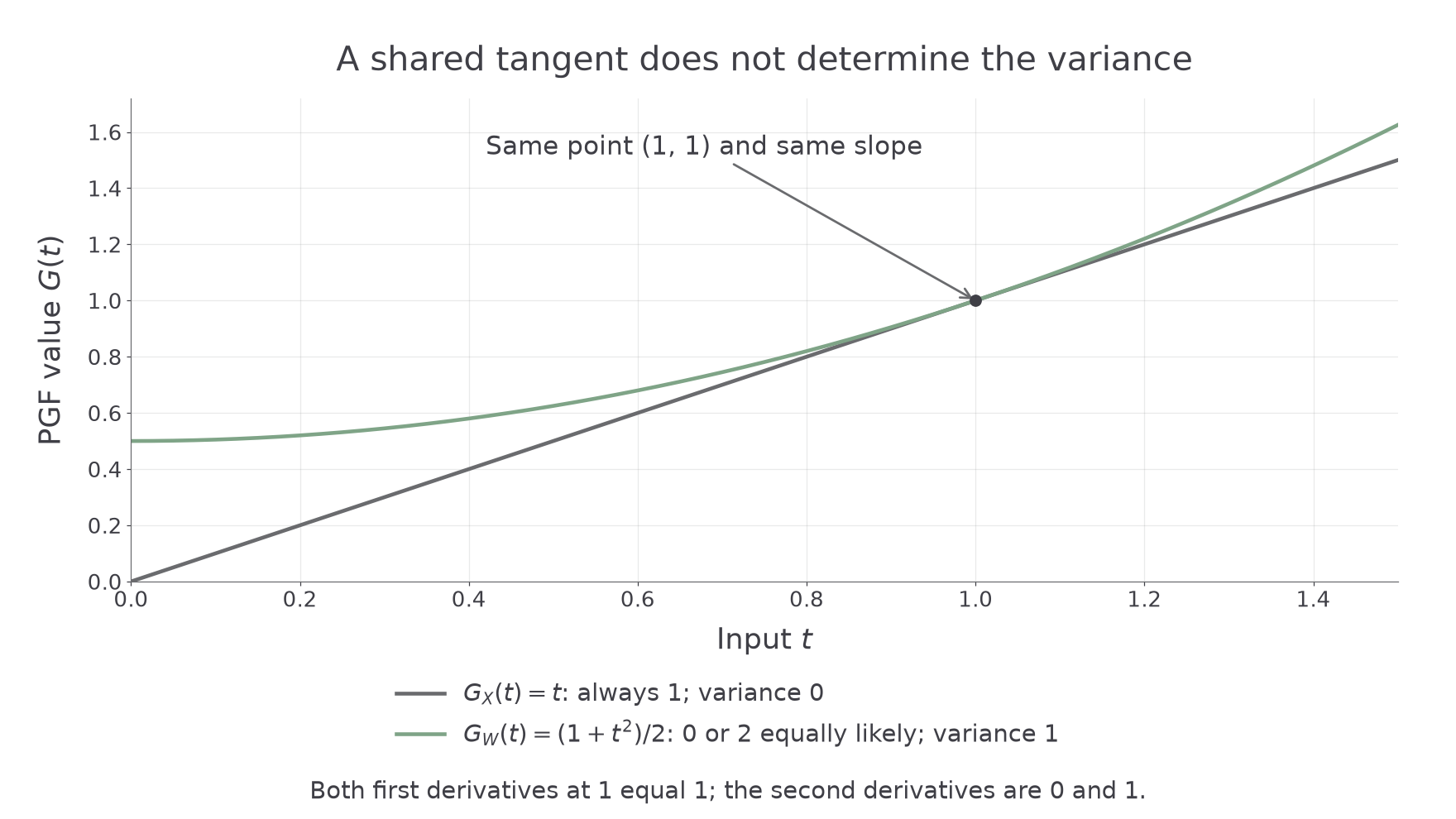
Two PGF curves pass through with the same slope. Must their distributions have the same variance?
Consider , which describes with certainty, and , which describes equally likely values and . Both have value and derivative at . Yet one distribution never varies and the other does. The second derivative will reveal what the shared tangent cannot.
You already know
A PGF is . Coefficients and derivative values at zero recover probabilities; moments use a different input. Recall , and use product and chain rules when differentiating.
For the distributions here, the necessary moments are finite and the PGF can be differentiated near . Write . Differentiating the series gives
Thus . Subtract the square of the mean to obtain the variance. This also explains why the second derivative alone is not the variance.
Moments from a PGF
Where the relevant moments exist,
The intermediate identity is . The mean and variance formulae are supplied; the displayed series argument justifies them.
In the formula booklet.
The two opening curves have the same height and slope at , but different bending. Their shared mean therefore leaves room for different variances.
[DIAGRAM: asset_name: Same PGF value and slope with different variance; asset_slug: 9fm0-fs114-shared-tangent; caption: PGFs can share their mean while their second derivatives reveal different spreads; description: A graph shows G X of t equals t in grey and G W of t equals one plus t squared over two in sage, for t from zero to one point five. Both curves meet at the marked point one comma one with the same tangent. The legend states that X is always one with variance zero, whereas W is zero or two equally likely with variance one. A note says both derivatives at one equal one, while the second derivatives at one are zero and one.]
Key idea
Differentiate first, then substitute . The second derivative supplies ; add the mean before subtracting its square.
Distinguish the three quantities in the following check.
Proving the binomial and Poisson moments
To prove a standard moment result using its PGF, show the derivatives, their values at one and the final variance simplification.
The booklet supplies both PGFs and their moments. A proof must connect them by calculus; quoting the target mean and variance is not a derivation.
Worked example 1: binomial moments from a polynomial power
Question. Use the PGF of to prove that its mean is and its variance is .
Plan. Write , differentiate twice and use .
Hence
Why this step? Substituting after differentiation makes the bracket equal without losing the powers of produced by the chain rule.
Answer. , , as required.
Check. At , the second derivative is zero and the variance reduces to the Bernoulli value . The degenerate case has both moments zero directly.
Worked example 2 changes the count model from binomial to Poisson. The derivative-at-one procedure stays the same; the exponential replaces the polynomial power.
Worked example 2: Poisson moments from an exponential
Question. Use the PGF of to prove that its mean and variance both equal .
Plan. Differentiate the exponential twice, then evaluate at one before simplifying.
Why this step? Each differentiation contributes another factor . The cancellation in the variance occurs only after adding the mean and subtracting its square.
Answer. and , as required.
Check. For , the derivative values are and , giving variance . These agree with the supplied Poisson moments.
Both pairs of moment results are in the formula booklet. The proofs explain their structure: the binomial variance retains a factor , while the Poisson variance equals its mean.
Watch out
Wrong: differentiate as . Right: include the inner derivative , then include another factor on the second differentiation. In a proof, unsupported target formulae do not replace these steps.
Use the exponential method with a specified parameter in this check.
Proving the waiting-time moments
Keep the successful-trial factor in a waiting-time PGF when differentiating: removing it changes the variable and its mean.
Write , with . The geometric trial-count PGF is . Its first derivative simplifies neatly if you combine the numerator terms before differentiating again.
Continue this lesson.
You’re previewing NovaLearn without an account. Create a free account to read the rest.
Create free account