FP1 2.1 - Taylor series
Build a power series around a point of your choice, rather than always around zero. You will derive the Taylor coefficients, expand explicit functions and obtain a local series from a differential equation without first solving it.
Moving the expansion point
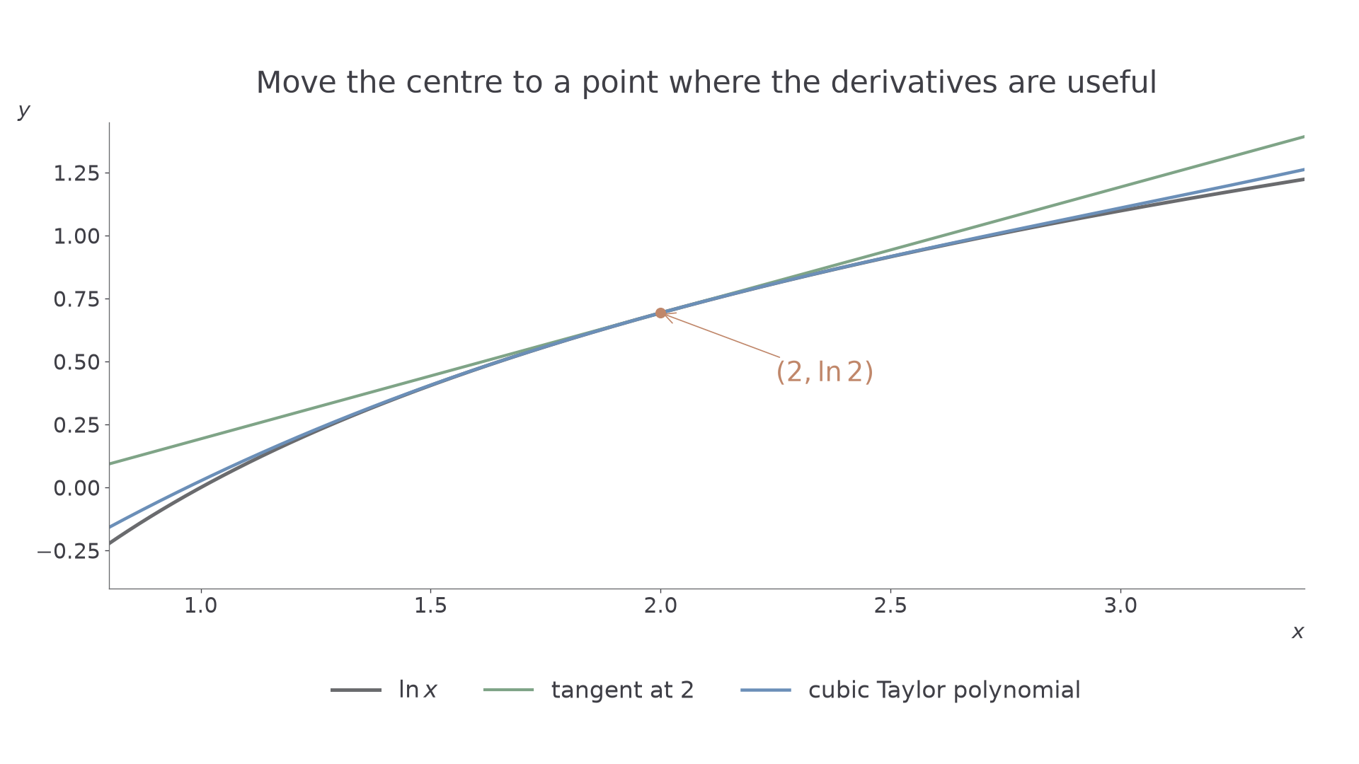
How can you approximate with a short polynomial when has no Maclaurin series at zero? Move the centre to . The small quantity becomes , and derivatives at replace the unavailable derivatives at zero.
You already know
A Maclaurin series has coefficient on . A finite truncation generally gives a local approximation. The full series must actually represent the function on the interval where you use it; infinitely many derivatives alone do not establish that representation.
Set . A power series about has the form . Since , evaluating at , where , gives
Thus moving the centre changes where the derivatives are evaluated, but not the factorial rule.
Taylor expansion about a
Where the Taylor series represents ,
The general term is . The expansion variable is , and every derivative coefficient is evaluated at . The booklet prints the zero-centre Maclaurin version; this shifted formula follows from it.
Not in the formula booklet: learn it.
The polynomial through degree matches the function's value and its first derivatives at the centre. It need not match the function far away. Use for a numerical truncation and retain an ellipsis when writing the start of an infinite series.
[DIAGRAM: asset_name: A Taylor polynomial centred at x equals 2; asset_slug: 9fm0-fp163-taylor-centre; caption: Derivatives at 2 produce a polynomial that follows the logarithm locally; description: A Cartesian graph shows ln x, the tangent ln 2 plus (x minus 2) over 2 and the cubic Taylor polynomial about x equals 2. Their common point (2,ln 2) is marked. The cubic follows the logarithm more closely near 2; the legend is outside the curves.]
Key idea
The centre determines both the powers and the derivative values . Move both together.
The next check separates the new expansion variable from the old one.
Expanding a trigonometric function about a non-zero point
Differentiate first, substitute the centre second and assemble the series last. A zero derivative value removes that power; it does not move the expansion point or shift the other factorials.
Worked example 1: sine about pi
Question. Derive the Taylor expansion of about , up to and including the term in .
Plan. Evaluate the function and its first three derivatives at , then use powers of .
Therefore
Why this step? The negative linear term comes from . Copying the Maclaurin sine coefficients unchanged would reverse the signs.
Answer. .
Check. , whose standard series is .
Change only the function from sine to cosine, keeping the centre and the highest permitted power.
Worked example 2: cosine about pi
Question. Derive the Taylor expansion of about through the term in .
Plan. Evaluate the cosine derivative cycle at the same centre.
Thus
Why this step? “Through the cubic term” asks you to account for that power, even when its coefficient is zero. It does not require inventing a non-zero cubic term.
Answer. The requested polynomial is ; the cubic coefficient is zero.
Check. , agreeing with the expansion.
The standard sine and cosine series are printed in the booklet. Their shifted expansions above are not separately printed; either derivative values or the angle-shift identities establish them.
Watch out
Wrong: write when expanding about . The function remains ; only the powers use the displacement .
Change the inner scale of cosine and keep the same centre.
Shifting a standard series and making an estimate
You can also introduce inside a familiar function and reuse its standard Maclaurin series. For a logarithm, extracting the centre as a factor makes the small quantity visible.
Continue this lesson.
You’re previewing NovaLearn without an account. Create a free account to read the rest.
Create free account