2.1.1(b)-(d) - Slide preparation, staining and drawings
This lesson teaches how a microscope observation becomes reliable evidence: prepare a thin slide, use stains sensibly, measure with calibrated scale, then communicate only what is visible. The focus is practical microscopy, not electron microscopy or organelle ultrastructure.
Preparing A Slide
For a plant wet mount, a thin epidermal peel avoids overlapping cell layers. With the lowest-power objective, use coarse focus to locate the specimen, centre it, then use fine focus after increasing power; avoid driving the objective into the coverslip. Adjust illumination for contrast. Handle glass and mounted needles carefully and use appropriate eye protection for the stain.
A smear is a different preparation: spread a small drop into a thin film with the edge of a second slide held at an angle, then allow it to air-dry before the specified fixation and staining. Prepared blood smears are used for observation; handling fresh human blood requires an approved laboratory procedure.
A light microscope works by passing visible light through, or reflecting light from, a specimen. For most cell work, the specimen must be thin enough for light to pass through and flat enough for structures to stay in one focal plane.
A common wet mount route is:
- Put a small, thin sample in a drop of water or mounting fluid on a clean slide.
- Lower a coverslip at an angle using a mounted needle.
- Blot away excess liquid.
- Start with low power, focus, then move to higher power only when the specimen is centred.
[DIAGRAM: slide_preparation_staining_measurement: Lesson 013: Light microscope slide preparation, staining and measurement - diagram 01; asset_slug: 013_m02_1_1_light_microscope_slide_preparation_staining_and_drawings__diagram_01; recommended_method: drawn_biology; description: Deterministic sequence showing thin sample, angled coverslip, stain drawn under the coverslip, and calibrated graticule measurement.]
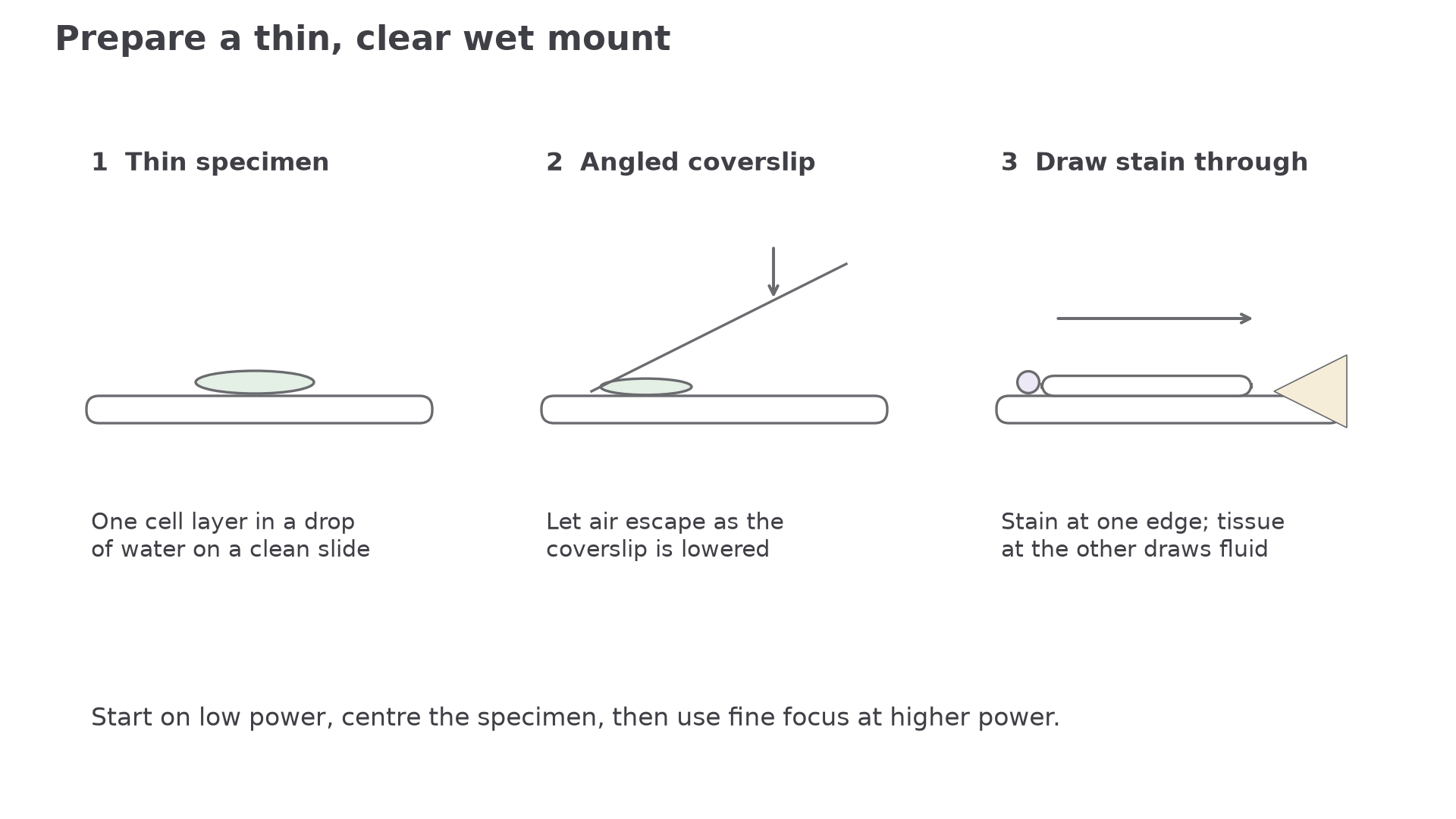
The coverslip keeps the sample flat and slows evaporation of the mounting fluid. Lowering it at an angle lets air escape rather than trapping bubbles.
Each step controls an artefact. A thick sample gives overlapping structures. A trapped air bubble can look like a circular cell part. Dust, fingerprints and excess stain can all create false evidence.
Using Stains
For example, methylene blue makes nuclei more distinct in cheek-cell preparations. In a prepared blood smear, a suitable differential stain gives contrasting nuclei and cytoplasm: a lobed, dark-stained nucleus supports identification of a white blood cell, while mammalian red blood cells lack nuclei. In a plant section, different cell-wall components can stain differently. The interpretation combines stain response with shape and position; staining does not improve the optical resolution of the microscope.
Many cells are almost transparent under a light microscope. A stain increases contrast, so boundaries and cell components are easier to distinguish. Staining is useful evidence, but it can alter or kill cells, so a stained slide is not always evidence of a living state.
Differential staining uses more than one staining effect to distinguish different cellular components or cell types. The important idea is not to memorise a catalogue of stains. It is that different parts of cells can take up stains differently because they contain different molecules or have different structures.
Useful examples:
| Staining idea | What it helps with | Evidence-based interpretation |
|---|---|---|
| A stain taken up by nuclei | locating cells and cell stages | darker-stained regions may identify nuclei |
| A differential stain in tissue | distinguishing cell types or tissue areas | different colours/intensities can support identification |
| Too much stain | obscures detail | method quality matters as much as adding dye |
When explaining a stain, link the method to evidence: "stain increases contrast so the structure can be distinguished", not just "stain makes it visible".
A dark object is not identified by darkness alone. Use an appropriate stain, its position within a visible cell and recognisable structure; also check for preparation artefacts.
Calibrating Measurements
An eyepiece graticule is a scale in the eyepiece. Its divisions have no fixed real size until calibrated. A stage micrometer has a known scale, usually in micrometres, so it can be used to find the real size represented by one eyepiece graticule division for a particular objective lens.
Calibration route:
- Place the stage micrometer on the microscope stage.
- Focus using the objective lens that will be used for the specimen.
- Align zero on both scales, then find a second matching point to measure a known stage distance and its corresponding graticule interval.
- Calculate the value of one eyepiece graticule unit.
- Replace the stage micrometer with the specimen slide and measure the specimen in graticule units.
Calibrating an eyepiece graticule
Calibrating A Graticule
With the ×40 objective, 50 eyepiece graticule divisions line up with 200 micrometres on the stage micrometer.
Value of one eyepiece division:
A cell is 18 eyepiece divisions wide.
Actual width:
The answer is 72 micrometres.
The calibration must be repeated if the objective lens changes, because the image size changes but the eyepiece scale stays physically the same.
Drawing Observations
A drawing has its own magnification; it need not equal the microscope’s magnification. A scale bar represents a known real distance and remains useful when the whole drawing is resized, because the bar and drawing enlarge together. Label the bar with its actual length and unit. For example, if a cell is measured as 50 µm wide and drawn 100 mm wide, a 20 mm line represents 10 µm.
A biological drawing is a scientific record, not an artwork. It should represent what is observed, not what a textbook says ought to be there.
[DIAGRAM: biological_drawing_conventions: Lesson 013: Evidence-based biological drawings from microscope observations - diagram 02; asset_slug: 013_m02_1_1_light_microscope_slide_preparation_staining_and_drawings__diagram_02; recommended_method: drawn_biology; description: Deterministic comparison of low-power tissue plan and high-power cell drawing, with scale bars, ruled labels and drawing-quality checklist.]
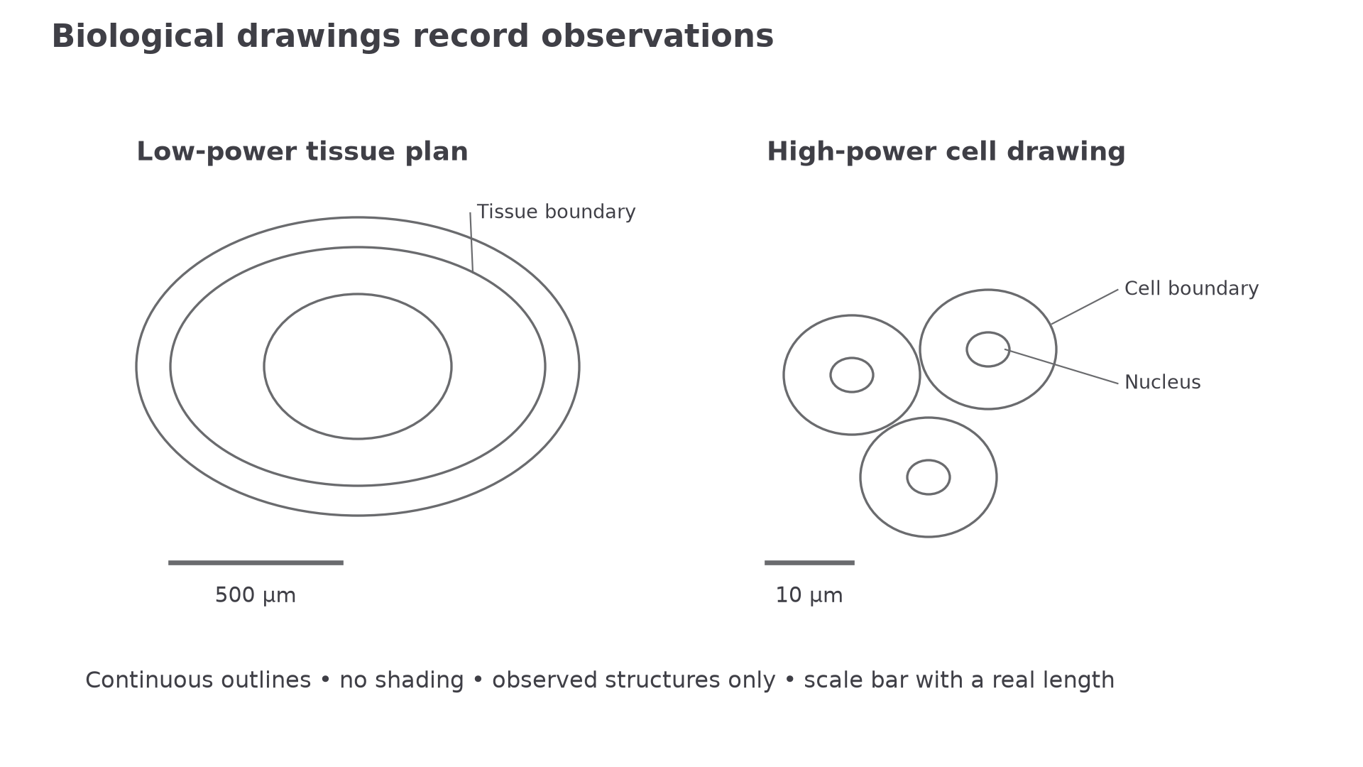
Low-power tissue plans show the distribution and boundaries of tissues. They should not include individual cell detail. High-power drawings may show individual cells and visible cell structures.
Good drawing conventions:
| Feature | Good practice | Common error |
|---|---|---|
| Lines | clear, single, continuous outlines | sketchy or shaded lines |
| Proportion | relative sizes match the view | enlarged favourite structures |
| Labels | horizontal labels with ruled lines touching the structure | crossed label lines or floating labels |
| Scale | scale bar or calibrated size | total magnification alone |
| Detail | only visible structures | invented organelles |
| Annotation | short note about an observed feature | long explanation of theory |
Quick Recap
Prepare a thin clean slide, interpret contrast cautiously, calibrate measurements for the objective used, and draw only observed features with valid size information.