1.1.3(a)-(d)(ii) - Analysis, calculations and graph skills
In this lesson you learn how experimental results become biological conclusions. You will process qualitative and quantitative results, choose suitable mathematical handling, use significant figures sensibly, and construct or interpret graphs with correct axes, scales, units, gradients and intercepts. The aim is not to make graphs look neat for their own sake; the aim is to make the pattern in the evidence clear enough to analyse.
From Results To Conclusions
An experimental result is the evidence collected from a practical. Some results are qualitative: they describe a change in words, such as "the solution became darker blue" or "the leaf disc floated". Other results are quantitative: they are numerical measurements, such as time, mass, length, absorbance, concentration or number counted.
Qualitative result
A descriptive observation that is not recorded as a numerical measurement.
Analysis begins after the result has been recorded. Processing means doing something useful to the raw result, such as calculating a mean, a rate, a percentage change, or plotting the values on a graph. Analysing means looking for the pattern shown by the processed results. Interpreting means explaining what that pattern suggests in the biological context.
A valid conclusion is a statement that follows from the results given. It should refer to the evidence and avoid claiming more than the method can show.
For example, suppose beetroot cylinders are left in water baths at different temperatures and the absorbance of the surrounding solution is measured.
| Temperature of water bath / °C | Absorbance of solution |
|---|---|
| 20 | 0.12 |
| 40 | 0.21 |
| 60 | 0.62 |
A weak conclusion would be: "High temperature destroys all membranes." That overclaims. A better conclusion is: "As temperature increased from 20 °C to 60 °C, absorbance increased from 0.12 to 0.62, suggesting more pigment leaked from the beetroot cells." This uses the data and keeps the claim tied to the experiment.
Move in order: raw result -> processed result -> pattern -> conclusion supported by the evidence.
Mathematical Handling And Significant Figures
Appropriate mathematical handling means choosing a calculation that answers the biological question. The calculation is not separate from the biology; it is how the pattern becomes measurable.
| Biological question | Useful mathematical handling |
|---|---|
| How fast is a process occurring? | Calculate a rate, often from change in y divided by change in x. |
| What is the central value of repeated readings? | Calculate a mean. |
| How large is the change compared with the starting value? | Calculate a percentage change. |
| Do two continuous variables show a relationship? | Plot a graph and interpret the trend or gradient. |
| Is a difference or correlation likely to be due to chance? | Select and use a suitable statistical test when that skill has been taught. |
For a mean, sum all included values and divide by their number. A percentage change is (final − initial) / initial × 100: a fall from 2.50 g to 2.20 g gives −12%, or a 12% decrease. Record why any value is excluded, and retain unrounded values until the final calculation.
This lesson does not teach every statistical test. The important habit here is to choose the mathematical tool that fits the data and the question.
Numerical notation expresses relationships precisely: = means equal, < less than, > greater than, ≪ much less than, and ≫ much greater than. The symbol ∝ means proportional to: if product amount is proportional to time, doubling time doubles the amount and a plot through the origin has a constant gradient. A straight line with a non-zero intercept is linear but is not directly proportional. The symbol ~ indicates an approximate value or relationship in this context; define its meaning when using it. For example, a cell length of ~20 µm is an estimate, not an exact measurement.
In standard form, write a number as a × 10ⁿ with 1 ≤ a < 10: 0.0050 = 5.0 × 10⁻³, retaining two significant figures. To check a result, estimate its scale: 0.39 divided by 3 is about 0.13, so 13 would signal a hundredfold error.
The median is the middle value in an ordered set, whereas the mode is the most frequent value. For times of 10, 12, 12, 14 and 32 s, the mean is 16 s, the median is 12 s and the mode is 12 s. The large final value pulls the mean upwards; choose a summary that answers the question and still report the variation rather than hiding the unusual value.
Significant figures are the digits in a number that carry meaning about precision. In biology, the final answer should not imply that the experiment was more precise than the measurements actually were. If a question tells you to give an answer to a particular number of significant figures, follow that instruction. If it does not, use a sensible number of significant figures based on the data supplied.
Rate And Significant Figures
A product concentration increases from 0.12 mmol dm⁻³ to 0.46 mmol dm⁻³ in 5.0 minutes.
Change in concentration = 0.46 - 0.12 = 0.34 mmol dm⁻³
Rate = change in concentration / time
Rate = 0.34 / 5.0 = 0.068 mmol dm⁻³ min⁻¹
The time and concentration change are given to 2 significant figures, so 0.068 mmol dm⁻³ min⁻¹ is a suitable final answer because it also has 2 significant figures.
Use units in the calculation, not just at the end. This helps you spot mistakes. If the y-axis is concentration in mmol dm⁻³ and the x-axis is time in minutes, then the gradient unit is mmol dm⁻³ min⁻¹.
Plotting Suitable Graphs
A suitable graph is chosen because it matches the type of data. The independent variable is normally placed on the x-axis because it is the variable deliberately changed or selected. The dependent variable is normally placed on the y-axis because it is the measured response.
Line graphs and scatter graphs show relationships between two quantitative variables; choose whether a line or curve is scientifically meaningful. A histogram instead shows frequencies of measurements grouped into continuous classes; when class widths differ, use frequency density so bar area represents frequency. Bar charts are more suitable when the independent variable is a set of categories. A graph should not be chosen just because it is familiar; it should reveal the relationship in the results.
In a scatter diagram, each point is one paired observation. An upward trend suggests positive correlation; a downward trend suggests negative correlation; a cloud with no trend shows no clear correlation. For example, if leaf area and water uptake both rise across sampled plants, they are positively correlated. This alone does not show that changing leaf area caused the difference: plant size or light exposure could affect both.
Good graph construction has four non-negotiable features.
| Feature | What it means |
|---|---|
| Quantity on each axis | The axis says what is being measured, such as time or concentration. |
| Unit on each axis where needed | The unit is included, such as min, cm, g, mmol dm⁻³. Absorbance and pH are dimensionless and need no unit. |
| Sensible scale | The scale is even, easy to read, increases conventionally, and lets the points use much of the grid. |
| Clear plotted points and best-fit line/curve | Points are visible and accurate; a trend line is not forced through the origin unless that is justified. |
The diagram shows the decisions often tested in graph questions: axes with quantities and units, a sensible scale, plotted points, a line of best fit, a gradient triangle and the y-intercept.
[DIAGRAM: graph_analysis_gradient_intercept: Lesson 3: Graph construction, gradient and intercept - diagram 01; asset_slug: 003_m01_1_3_analysis_mathematical_handling_and_graph_skills__diagram_01; recommended_method: drawn_biology; description: A clean 16:9 drawn graph showing labelled axes with units, plotted experimental points, a straight line of best fit, a large gradient triangle labelled change in y and change in x, and the y-intercept c at x = 0.]
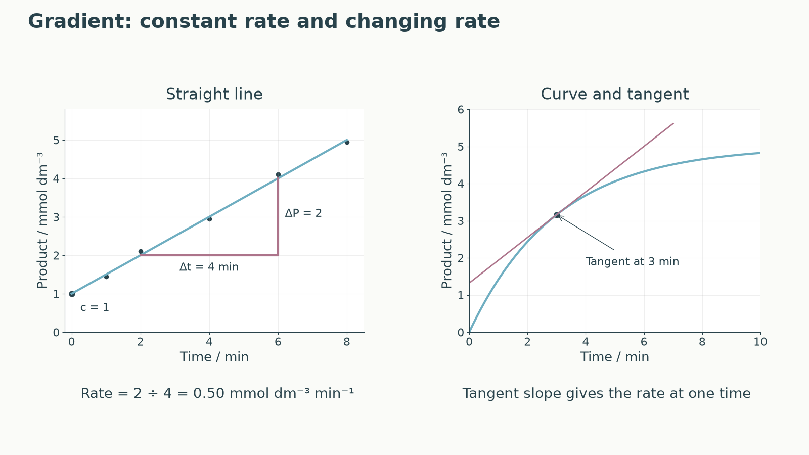
A common exam error is joining every point dot-to-dot when a clear overall trend exists. Another is forcing a line through the origin because it "looks scientific". The line or curve should represent the trend in the experimental results, with a reasonable balance of points around it.
Gradients And Intercepts
On a straight-line graph, the equation
Linear relationship
means that y changes linearly with x. The gradient is m. It tells you how much y changes for each unit change in x. The intercept is c. The y-intercept is the value of y when x = 0.
To calculate a gradient, use two points on the line of best fit. They should be far apart, because a small triangle magnifies reading errors. Do not use raw data points unless they actually lie on the best-fit line.
Gradient
Suppose a line of best fit for product concentration against time passes through these points on the line:
- (1.0 min, 1.80 mmol dm⁻³)
- (6.0 min, 5.30 mmol dm⁻³)
Gradient And Intercept
Gradient = change in y / change in x
Gradient = (5.30 - 1.80) / (6.0 - 1.0)
Gradient = 3.50 / 5.0 = 0.70 mmol dm⁻³ min⁻¹
Using y = mx + c and the point (1.0, 1.80):
1.80 = (0.70 × 1.0) + c
c = 1.10 mmol dm⁻³
The y-intercept is therefore 1.10 mmol dm⁻³. In this context, it is the estimated product concentration when time is 0 min, based on the best-fit line.
For a curved graph, the gradient changes along the curve. To estimate an instantaneous rate at a stated time, draw a tangent that follows the curve at that point, then use two widely separated points on that tangent. A chord joining two points on the curve gives an average rate over that interval, not the instantaneous rate. A nearly horizontal tangent indicates a rate close to zero.
When you report a gradient, include the unit made from the y-axis unit divided by the x-axis unit. When you report an intercept, use the y-axis unit because the intercept is a y-value.
Interpreting a sampled optimum
Data interpretation usually rewards three habits: state the pattern, use evidence, and keep the conclusion valid. A description says what the data show. A calculation processes the data. A conclusion says what the data suggest in the biological context.
The command word matters. If asked to "Describe", focus on the pattern and use values. If asked to "Calculate", show the method and units. If asked to "Conclude" or "Interpret", connect the pattern to the biological meaning without claiming more than the results allow.
For example:
| pH | Mean rate of reaction / arbitrary units min⁻¹ |
|---|---|
| 5 | 1.2 |
| 6 | 2.8 |
| 7 | 5.4 |
| 8 | 3.1 |
| 9 | 0.9 |
A description is: "The rate increases from pH 5 to pH 7, then decreases from pH 7 to pH 9." A data-supported conclusion is: "The enzyme has the highest mean rate at pH 7 in these results, so pH 7 is closest to the optimum among the pH values tested." Avoid saying "the optimum is exactly pH 7" unless the experiment tested enough values to support that precision.
When using data, quote enough values to support the point. Do not just say "it went up" when a comparison with numbers is available.