E10.8 - Cumulative frequency, quartiles and percentiles (Extended)
A frequency table counts observations in separate intervals. How can you find the time below which three quarters of all journeys lie? E10.8 accumulates those counts, draws a smooth cumulative frequency curve and uses it to estimate the median, quartiles, interquartile range and percentiles.
Cumulative frequency tables
Suppose 5 journeys take at most 10 minutes and another 15 take more than 10 but at most 20 minutes. Then journeys take at most 20 minutes. A cumulative total includes every earlier class.
Cumulative frequency
Cumulative frequency is the number of observations up to a specified boundary. Add frequencies successively. The final cumulative frequency is the total number of observations, , and the totals cannot decrease.
Preserve the table's boundary convention. For , the cumulative count at 20 includes 20. For , it counts values less than 20.
Worked example 1: accumulating journey times
Question. Complete the cumulative frequencies for these 80 journeys.
| Time (minutes) | ||||
|---|---|---|---|---|
| Frequency | 5 | 15 | 25 | 35 |
Plan. Keep a running total, attaching each total to its upper boundary.
Answer. At 10, 20, 30 and 40 minutes, the cumulative frequencies are 5, 20, 45 and 80.
Check. Successive differences give back 5, 15, 25 and 35. The final total equals all 80 journeys.
The second distribution has five classes. More classes simply mean more running totals.
Worked example 2: a second distribution
Question. Lengths , in centimetres, have frequencies 4, 12, 20, 28 and 36 in , , , , . Complete the cumulative table and find the total.
Plan. Add each new frequency to the previous cumulative total.
Answer. Cumulative counts 4, 16, 36, 64, 100; total .
Check. The final two cumulative counts differ by , the last class frequency. None of the totals decreases.
Do not add cumulative totals together to find the sample size: that repeatedly counts the same observations.
Drawing cumulative frequency curves
Plot each cumulative count at the boundary it describes, using the data variable horizontally and cumulative frequency vertically. Include zero at the lowest boundary when no observations lie below it. Mark clear crosses and join them with a suitable smooth, non-decreasing curve.
Watch out
Class midpoints are used for estimated means, not for cumulative plotting. A cumulative count of 20 at an upper boundary of 20 minutes belongs at , rather than at the class midpoint .
For rounded measurements, use actual class boundaries when appropriate. Heights rounded to the nearest centimetre and grouped as 10–19 cm have boundaries 9.5 and 19.5 cm. Plot the cumulative count for that class at 19.5, not 19 or its midpoint 14.5.
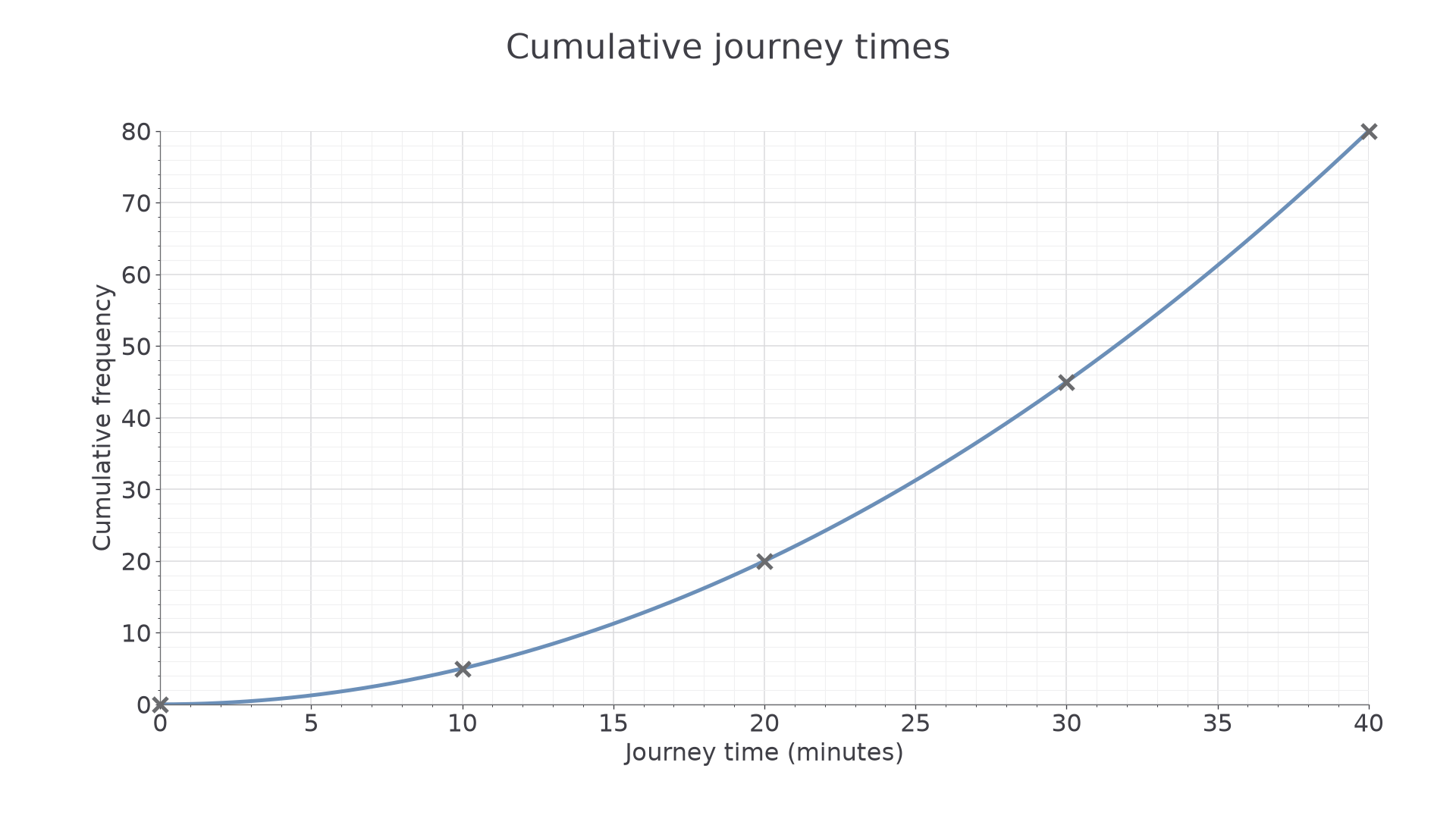
[DIAGRAM: asset_name: Cumulative journey times; asset_slug: cumulative_journey_times; caption: Crosses at upper boundaries build a smooth curve for 80 journeys.; description: A labelled grid plots (0,0),(10,5),(20,20),(30,45),(40,80) with clear crosses and a smooth increasing curve. The horizontal axis is journey time in minutes; the vertical axis is cumulative frequency, scaled 0 to 80.]
Worked example 3: plotting the journey curve
Question. Draw a cumulative frequency curve using totals 5, 20, 45, 80 at upper time boundaries 10, 20, 30, 40 minutes. No journey takes zero minutes or less. Estimate how many take at most 25 minutes.
Plan. Include the starting point, plot boundary-count pairs, then read up from 25 to the smooth curve and across.
Plot . The illustrated curve passes through these crosses without falling between them. At 25 minutes it reads approximately 31 on the cumulative scale.
Answer. The curve is shown; about 31 journeys take at most 25 minutes.
Check. This lies between 20 journeys at 20 minutes and 45 journeys at 30 minutes. An answer below 20 or above 45 would conflict with the known totals.
The next graph has a larger total and a longer horizontal range. Choose its scale from these data, rather than copying the first graph unchanged.
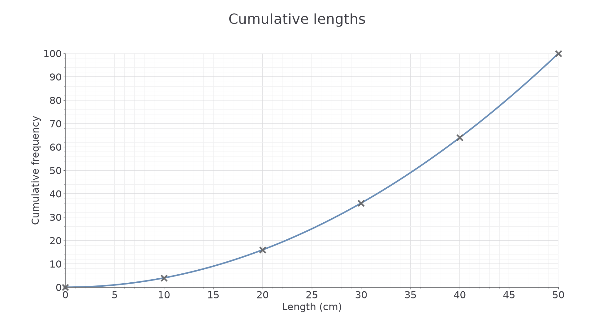
[DIAGRAM: asset_name: Cumulative lengths; asset_slug: cumulative_lengths; caption: The length curve ends at a cumulative total of 100.; description: A labelled grid plots (0,0),(10,4),(20,16),(30,36),(40,64),(50,100) with clear crosses and a smooth increasing curve. Length in centimetres is horizontal and cumulative frequency is vertical.]
Worked example 4: reading a complementary count
Question. Draw the length curve for cumulative counts 4, 16, 36, 64, 100 at upper boundaries 10, 20, 30, 40, 50 cm. No length is zero or less. Estimate the number longer than 35 cm.
Plan. Plot the boundary pairs with , read the count at or below 35, then subtract from the total.
The illustrated smooth curve reads about 49 at 35 cm. Therefore
Answer. About 51 lengths.
Check. The count longer than 30 cm is 64; the count longer than 40 cm is 36. A count of 51 at the intermediate boundary fits these bounds.
Smooth curves represent estimates within classes: different reasonable curves can give slightly different readings. Use the grid scale carefully, within half the smallest square, and round a count sensibly to whole observations.
Continue this lesson.
You’re previewing NovaLearn without an account. Create a free account to read the rest.
Create free account