C3.2; E3.2 - Graphs, tables and windows on a calculator | Cambridge IGCSE International Mathematics

A calculator screen looks empty after you enter $y=(x-12)^2-4$ . Is there really no graph? C3.2 and E3.2 use graph entry, tables and point plotting to choose a useful view and transfer the mathematics clearly to paper.

Graph entry and window

A graphic display calculator shows only a rectangular window of the coordinate plane. A correct function can lie outside that rectangle. Check the entry first, then choose horizontal and vertical limits that show the required input interval and the important shape.

Graph window

A graph window specifies the smallest and largest displayed $x$ -values and $y$ -values. Each axis has its own scale. The window changes what you see; it does not change the function.

Open the graphing facility, enter the function as $Y_1$ or the equivalent on your model, set the four limits and draw. Use brackets to preserve a whole squared bracket, numerator or denominator. Check one easy input independently if the screen looks unexpected. Key names vary between models, so learn where your own calculator sets graph and table options.

This lesson uses the permitted graph, table and point-plotting features. Later work uses graph zeros, local maxima/minima and intersections. Other built-in applications gain no credit, and symbolic algebraic logic or external programs are not permitted. A graphic display calculator is required on Papers 3–6; calculators are prohibited on Papers 1 and 2.

Worked example 1: a visible quadratic

Question. Use a GDC to sketch $y=x^2-4$ for $-3\le x\le3$ . Give a suitable window and justify it.

Plan. Check a few outputs, then choose a vertical range containing the low point and endpoint heights.

\begin{aligned} x=-3&\quad\Longrightarrow\quad y=9-4=5\\ x=0&\quad\Longrightarrow\quad y=-4\\ x=3&\quad\Longrightarrow\quad y=5 \end{aligned}

Enter $Y_1=x^2-4$ . One suitable window is $x_{\min}=-3$ , $x_{\max}=3$ , $y_{\min}=-5$ , $y_{\max}=6$ . The graph is an upward curve with low point $(0,-4)$ , passing through $(-3,5)$ , $(3,5)$ , $(-2,0)$ and $(2,0)$ .

Answer. Use the stated window and sketch the symmetric upward curve with labelled axes, vertex and intercepts.

Check. Squaring cannot give a negative value, so $x^2-4\ge-4$ . On this interval $x^2\le9$ , so no output exceeds 5. The chosen window contains the whole required piece.

Move the same shape 12 units along the input scale next. An unchanged default window can now miss it completely.

Worked example 2: moving the viewing window

Question. Use a GDC to sketch $y=(x-12)^2-4$ for $9\le x\le15$ . Explain why the window $-3\le x\le3$ , $-5\le y\le6$ would not show this required piece.

Plan. Group $x-12$ before squaring and centre the horizontal window on the required interval.

\begin{aligned} x=9&\quad\Longrightarrow\quad y=(-3)^2-4=5\\ x=12&\quad\Longrightarrow\quad y=-4\\ x=15&\quad\Longrightarrow\quad y=5 \end{aligned}

Enter $Y_1=(x-12)^2-4$ . Use $9\le x\le15$ , $-5\le y\le6$ . The low point is $(12,-4)$ , and the graph crosses the $x$ -axis at 10 and 14.

Answer. The new window shows the required upward curve. The old horizontal range excludes every input in the requested interval, so it cannot show that piece.

Check. Substituting 10 and 14 gives $(-2)^2-4=0$ and $2^2-4=0$ . At the old screen's rightmost input 3, the output is 77, above its vertical range as well.

[DIAGRAM: asset_name: The same graph in two windows; asset_slug: gdc_window_choice; caption: An empty window can hide a valid graph; choose limits around the required interval.; description: Two accurate grids show y equals x minus twelve all squared minus four. The left window spans x minus three to three and y minus five to six and contains no portion of the graph. The right spans x nine to fifteen and the same vertical limits, showing the whole requested parabola with labelled vertex twelve comma minus four, roots ten and fourteen, and endpoints at nine comma five and fifteen comma five. The limits are printed above each panel.]
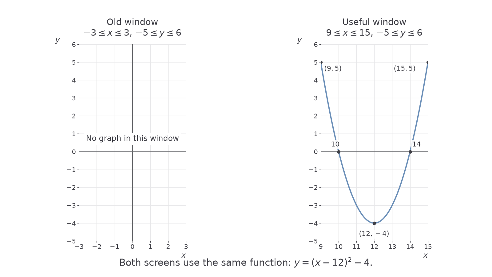
An empty window can hide a valid graph

A graph may look narrow or wide because the two axes use different screen scales. Read the scale before interpreting a shape. Zooming out indefinitely can hide useful detail just as a narrow window can omit it.

The same steps work for an unfamiliar supplied rule. For $y=\sqrt{x+4}-2$ , enter the whole $x+4$ under the square root, using the root template or brackets in a linear entry. On the supplied interval $-4\le x\le5$ , the inputs $-4,0,5$ give outputs $-2,0,1$ , so a useful window is $-5\le x\le6$ , $-3\le y\le2$ . The graph starts at $(-4,-2)$ ; a real-valued entry has no output when $x+4<0$ , so the extra space to the left of $-4$ stays empty. Check the entry at $x=0$ : $\sqrt{0+4}-2=0$ .

Watch out

An empty screen is evidence about a window, not proof that a function has no values. Check the expression, the required input interval and some sample outputs before changing limits.

Choose a view from the given interval and outputs.

Tables

A calculator's table lists outputs for selected inputs of an entered function. Set the start input, step size and end input, or use the model's equivalent list of chosen inputs. A step of 0.5 means the inputs increase by 0.5; it does not fix the changes in the outputs.

Table of values

A table of values pairs selected inputs $x$ with the corresponding outputs $f(x)$ . Each row or column gives a point $(x,f(x))$ on the graph.

Read both entries of a pair. A display showing a rounded decimal output may conceal extra precision: retain the stored value and round only the requested final answer. A table samples inputs; it does not list every value on a continuous curve.

Worked example 3: unit steps

Question. Use a GDC table for $f(x)=x^2-x-2$ , starting at $-1$ , ending at 2, in steps of 1.

Plan. Enter the rule and table settings, then check the first pair by substitution.

f(-1)=(-1)^2-(-1)-2=0

$x$	$-1$	0	1	2
$f(x)$	0	$-2$	$-2$	0

Answer. The table is shown above, with points $(-1,0)$ , $(0,-2)$ , $(1,-2)$ and $(2,0)$ .

Check. Reverse the last two operations: adding $x+2$ to each listed output gives $1,0,1,4$ . These are the squares of the corresponding inputs $-1,0,1,2$ , so every pair satisfies $y+x+2=x^2$ .

Keep the same rule and interval but halve the step. The extra inputs reveal the bottom of the curve between the earlier samples.

Continue this lesson.

You’re previewing NovaLearn without an account. Create a free account to read the rest.

Create free account

Last Accessed

Number

Algebra

Geometry

Mensuration

Trigonometry

Coordinate geometry

Functions

Transformations and vectors

Probability

Statistics

Investigation and modelling

C3.2; E3.2 - Graphs, tables and windows on a calculator

Graph entry and window

Tables

Continue this lesson.

Learn faster with Nova