C10.2; E10.2 - Comparing data and judging conclusions
Two groups can have the same average while behaving very differently. What evidence would make “more reliable” a fair description of one group? C10.2 and E10.2 combine averages, spread, tables and graphs to make supported comparisons and recognise restrictions on conclusions.
Comparing distributions
An average describes a typical value, while spread describes variation. A useful comparison often needs both: a delivery service can be faster on average but less consistent. State which measure supports each part of your conclusion, with the variables and units.
You already know
The mean uses every value and can be pulled by an extreme observation. The median describes the centre of ordered data. Range uses the two extremes; IQR describes the width of the middle half and is less affected by extreme observations.
Choose measures suited to the data and the question. Compare like quantities in the same units, and distinguish “smaller” from “better”: a smaller delivery time is desirable, whereas a smaller test score usually is not.
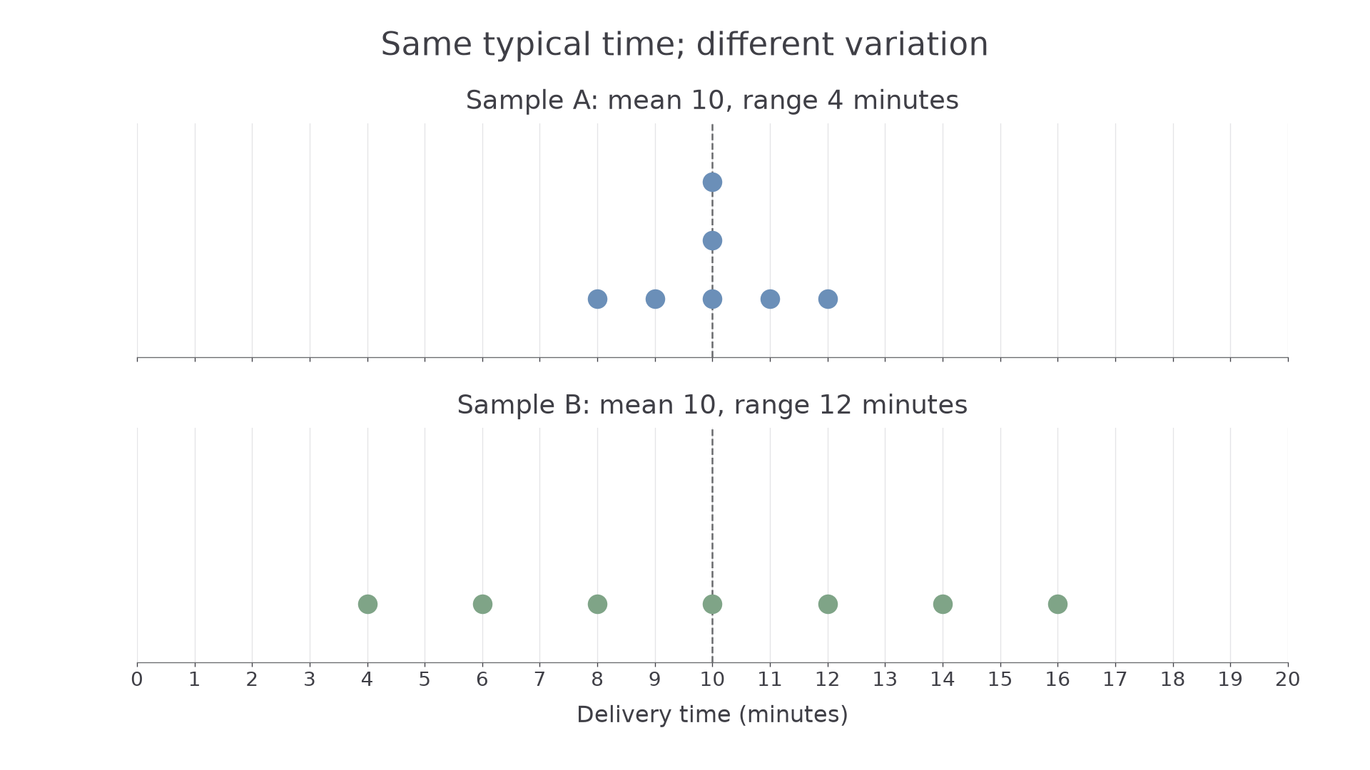
[DIAGRAM: asset_name: Same centre different spread; asset_slug: comparing_dot_plots; caption: Both delivery samples have mean and median 10 minutes, but B has the greater range.; description: Two stacked dot plots on the same 0 to 20 minute scale show A values 8,9,10,10,10,11,12 and B values 4,6,8,10,12,14,16. Repeated tens in A are stacked and both samples have seven observations.]
Worked example 1: the same average
Question. Compare delivery times A: minutes and B: minutes, using mean and range.
Plan. Calculate each average and each spread, then link both to delivery times.
Answer. Both samples average 10 minutes. A's times are more consistent by range because 4 minutes is smaller than B's 12 minutes; neither has the smaller mean.
Check. Each sample is symmetric around 10, checking the equal means. The shared-scale plots show B extending farther in both directions.
The next comparison changes the centres as well as the spreads, so there is a trade-off rather than one group winning on both measures.
Worked example 2: typical value and consistency differ
Question. Machine A has median completion time 20 seconds and IQR 4 seconds. Machine B has median 18 seconds and IQR 9 seconds. Compare typical time and consistency.
Plan. Use medians for typical time and IQRs for the middle half's variation.
Answer. B typically finishes 2 seconds sooner by median. A is more consistent for the middle half of times because its IQR is 5 seconds smaller.
Check. A larger spread is not automatically a longer typical time: B has the smaller median but larger IQR. Neither measure implies that every B run is faster than every A run.
The opening reliability claim needs a stated meaning. If reliability means less variable times, use a suitable measure of spread; an average alone cannot establish it.
Reading inferences
A conclusion should follow from the displayed information, rather than from the visual size of a bar or the larger of two counts. If group sizes differ, compare proportions or percentages when the question concerns how common an outcome is.
Supported inference
A supported inference is a conclusion justified by the available data and their context. It can describe a sample or suggest a pattern, but its certainty and scope must match the evidence.
First identify the relevant numerator and denominator. Check that categories, units and definitions are comparable, then describe the resulting difference without adding a cause the data did not establish.
Worked example 3: preferences in unequal groups
Question. In a survey, 18 of 30 morning students and 24 of 60 afternoon students prefer online revision. Compare the proportions preferring online revision.
Plan. Divide each preference count by its own group total.
Answer. A greater proportion of the morning sample prefer online revision: 60% compared with 40%, a difference of 20 percentage points.
Check. The morning group is half the size of the afternoon group. Doubling its count gives 36 of 60, greater than 24 of 60, confirming the comparison despite its smaller raw count.
Continue this lesson.
You’re previewing NovaLearn without an account. Create a free account to read the rest.
Create free account