E9.2, E9.6 - Cumulative frequency and percentiles
Grouped counts can show approximately where the middle observations lie, even when their exact values are hidden. You will build cumulative frequency tables and smooth curves, read median and percentile estimates, and compare distributions using median and interquartile range.
Cumulative totals and class boundaries
If eighty journeys have been grouped into time intervals, how can you estimate the time by which half the journeys were completed? Add the counts as you move through the intervals: that running total connects a time to the number completed by then.
Cumulative frequency
A cumulative frequency is a running total of frequencies up to a stated boundary. For the adjoining classes , and so on, the cumulative frequency at twenty counts all observations with .
Use the upper class boundaries for the running totals, and include a starting point of zero frequency at the lowest boundary. A cumulative total cannot decrease: extending the threshold cannot remove observations already counted.
Worked example 1: building the running totals
Question. Complete the cumulative frequencies for these eighty journey times.
| Time , minutes | Frequency | Upper boundary | Cumulative frequency |
|---|---|---|---|
Plan. Begin at zero, add each class frequency, and attach the result to that class's upper boundary.
Here means the cumulative count at twenty minutes; it is a short way to label a running total.
Answer. The cumulative frequencies are , with starting point .
Check. Successive differences recover the original frequencies: for example, . The final cumulative total equals .
Now work backwards from cumulative counts to an interval count. A cumulative count at forty already includes everything counted at twenty.
Worked example 2: subtracting cumulative counts
Question. Using the same table, find the number of journeys with and the number longer than forty minutes.
Plan. Subtract the earlier total from the later one; use the overall total for the upper tail.
Answer. Forty-eight journeys are longer than twenty and at most forty minutes; eight are longer than forty minutes.
Check. The interval combines the third and fourth classes: . The final class alone contains eight, confirming the upper-tail count.
For measurements rounded to the nearest unit, class labels may differ from their actual boundaries. Recorded whole-minute classes –, – and – meet at and minutes, not at gaps between ten and eleven. Their lowest and highest outer boundaries are and . Use these boundaries when drawing a curve for the underlying continuous measurement.
Watch out
Do not plot a running total against a class midpoint: it counts observations up to the upper boundary. Also distinguish “longer than forty” from “at most forty”; the latter is the cumulative count itself.
Build and subtract new cumulative totals.
Drawing a cumulative frequency curve
A cumulative frequency curve plots the running totals against the class boundaries. Label the horizontal measurement axis with its unit and the vertical axis “Cumulative frequency”. Choose scales that include the lowest boundary, all upper boundaries and the total frequency.
Mark clear crosses and join them with a smooth nondecreasing curve. Do not draw separate bars or a descending section. The values between boundaries are estimates: grouping has hidden the exact positions of the observations.
Worked example 3: continuous class boundaries
Question. Draw the cumulative frequency curve for the eighty journey times in Part 1.
Plan. Plot the zero starting point and each upper-boundary total, then draw one smooth rising curve through them.
Answer. The left panel below shows all six crosses joined by a smooth nondecreasing curve.
Check. Its final height is eighty. Its greatest rise is from twenty to thirty minutes, where the original table places the greatest frequency, thirty-two. A curve rising most steeply in an empty class would contradict the data.
Change the presentation to recorded whole-minute classes. The running-total method stays the same, but the continuous class boundaries are half a minute beyond the integer labels.
Worked example 4: rounded measurements
Question. Times recorded to the nearest minute are grouped as –, – and – minutes, with frequencies . Draw their cumulative frequency curve using continuous class boundaries.
Plan. Use boundaries , then attach cumulative totals zero, four, sixteen and twenty.
Answer. The right panel uses the continuous boundaries and a smooth nondecreasing join.
Check. The middle section rises by , matching the middle class frequency. The adjoining class boundaries coincide at and , so the underlying time intervals leave no gap.
[DIAGRAM: asset_name: Drawing cumulative curves at boundaries; asset_slug: cumulative_construction; caption: Plot upper-boundary totals, with a zero-frequency starting point.; description: The left panel has Journey time minutes from zero to fifty and Cumulative frequency from zero to eighty, six marked crosses at zero zero ten eight twenty twenty-four thirty fifty-six forty seventy-two fifty eighty and a smooth nondecreasing curve. The right panel has Recorded time continuous boundaries minutes from zero point five to thirty point five and Cumulative frequency zero to twenty, with crosses zero point five zero ten point five four twenty point five sixteen thirty point five twenty joined smoothly. Both panels have complete numerical scales.]
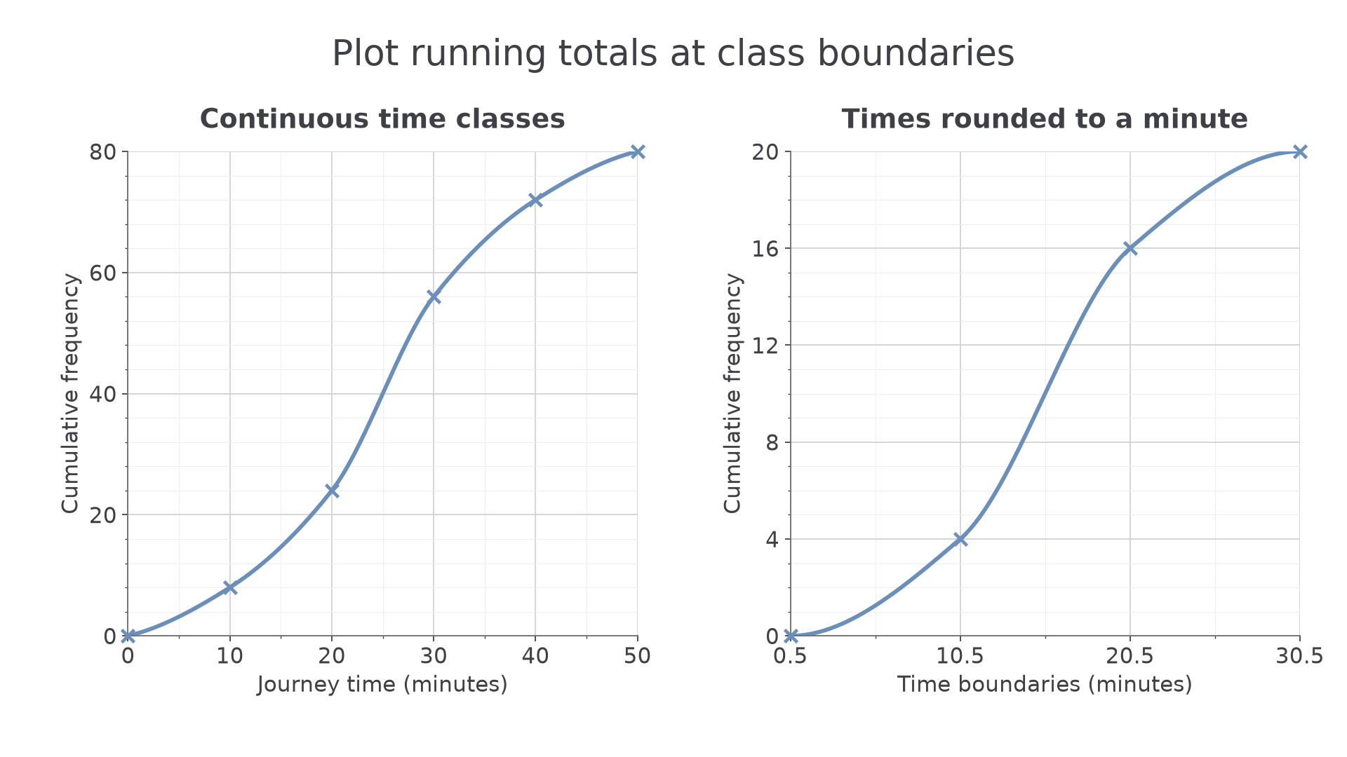
The two scales differ, but the construction is the same: boundaries horizontally, accumulated counts vertically. A steeper stretch means observations accumulate more quickly over that measurement interval.
Exam tip
Plot every required point clearly, then use a smooth curve rather than straight segments with sharp corners. Your curve must keep increasing or stay level; it cannot lose observations as the threshold increases.
Construct a curve from a fresh cumulative table on the supplied axes.
Reading medians, percentiles and quartiles
A percentile identifies a position in an ordered distribution. The percentile is the value at cumulative frequency , where is the total frequency. About of the observations lie at or below it. On a grouped curve this is an estimate, and ties or rounding can affect the exact proportion.
Continue this lesson.
You’re previewing NovaLearn without an account. Create a free account to read the rest.
Create free account