E2.11, E3.2, E3.5 - Linear equations in different forms
Different-looking equations can describe the same straight line. You will rearrange and obtain line equations for E3.5, draw their graphs for E3.2, and recognise and sketch the linear family in E2.11. Choosing a useful form makes gradients, intercepts and special cases easier to see.
Rearranging a linear equation
Do and describe different lines? At first they look different, but subtracting and dividing by transforms the first into the second without changing which coordinate pairs satisfy it.
General linear equation
A straight-line equation can be written as
where , and are constants and are not both zero. The terms contain only first powers of and , with no product . In this lesson the coefficients are rational numbers.
If , isolate by subtracting from both sides and dividing every term by . This gives . You can then read the gradient and y-intercept. The letters here name the coefficients in the general form; the constant on the right is not automatically the y-intercept.
Worked example 1: a positive y-coefficient
Question. Rearrange into . State its gradient and y-intercept.
Plan. Leave the -term alone, then divide the whole equation by its coefficient.
Answer. , with gradient and y-intercept .
Check. Multiplying the final equation by and adding returns . At , the original gives , confirming the intercept .
Change only the sign of the -coefficient. Dividing by a negative number changes the signs of both terms on the other side.
Worked example 2: a negative y-coefficient
Question. Rearrange into . State its gradient and y-intercept.
Plan. Isolate , then divide every term by .
Answer. , with gradient and y-intercept .
Check. Substitute : the original gives , and the rearranged equation gives . Reversing the rearrangement also returns the original equation.
When , the condition on the coefficients forces . Then gives the vertical line ; dividing by would be invalid. When and , the equation gives the horizontal line . For example, means , while means .
If both coefficients were zero, would describe every point in the plane, and would describe no points. Neither is one straight line. This is why the definition excludes that pair of coefficients.
Watch out
From , the line is wrong: it divides the second term by but loses the sign change in the first. Divide every term by the same non-zero number.
A different coefficient gives this fresh check.
Drawing and sketching different forms
The graph of contains all coordinate pairs satisfying that equation. You can rearrange to and make a table, just as before. Another efficient choice is to find the two axis intercepts: on the -axis, ; on the -axis, .
A drawn graph needs labelled axes, even numbered scales and accurately plotted points joined with a ruler. A sketch shows the line's direction, axis crossings and other important features with labels; its distances need not be to scale. Even a sketch must show a positive crossing on the positive side of the axis.
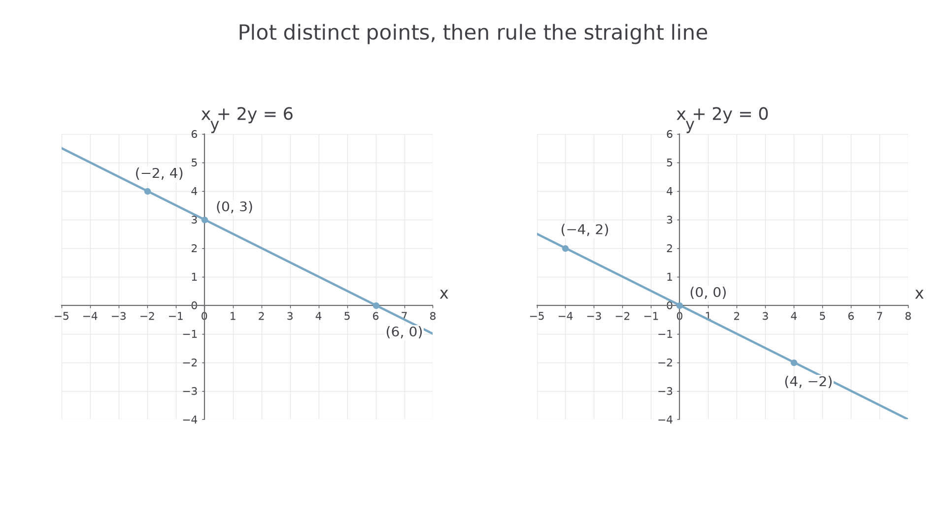
[DIAGRAM: asset_name: Plotting general line equations; asset_slug: general_line_plotting; caption: Two intercepts fix the left line; the line through the origin needs another distinct point.; description: Two equal-scale numbered grids. The left plots x plus two y equals six through zero comma three, six comma zero and negative two comma four. The right plots x plus two y equals zero through negative four comma two, zero comma zero and four comma negative two. Each line is extended across its grid.]
Worked example 3: using distinct intercepts
Question. Find the axis intercepts of , then draw its graph on suitable axes.
Plan. Set one coordinate to zero at a time, then use a third point as a check.
Answer. Plot , and on numbered axes, then rule and extend the line through them, as shown on the left.
Check. From to , a run of gives rise . From to , a run of gives rise . Both give gradient .
Change only the constant on the right from to . Both intercept calculations now return the origin; they have not supplied two distinct points.
Worked example 4: a line through the origin
Question. Find three points on , then draw its graph.
Plan. Use the origin and choose two non-zero inputs, rather than counting the origin twice.
Answer. Plot , and , then rule and extend the line, as shown on the right. A sketch would label the axes and origin and show the line falling through quadrants II and IV.
Check. Rearranging gives : the gradient is and the y-intercept is zero, agreeing with the drawn line.
Continue this lesson.
You’re previewing NovaLearn without an account. Create a free account to read the rest.
Create free account