E2.10, E2.11 - Turning points and growth models
An algebraic form can reveal a graph feature that a long table only estimates. You will find quadratic turning points by completing the square for E2.11, then draw and interpret exponential growth and decay and solve model equations by intersections for E2.10.
A quadratic turning point from completed square
Can you locate a quadratic's lowest point without plotting dozens of values? A square supplies the answer: it is never negative. Completing the square puts this fact where you can use it.
For example, is always at least , because the squared term contributes zero or a positive amount. Its least output is , reached when . This identifies the point exactly.
Completed-square form
For a quadratic written as
the turning point is , and the symmetry line is . If , it is a minimum; if , a maximum. Not given in the List of formulas: learn the connection to a non-negative square.
The sign inside the bracket is reversed in the turning point's first coordinate: gives . The constant outside the squared expression gives its height. If the coefficient of is not one, factor it out of the squared and linear terms before completing the square.
[DIAGRAM: asset_name: Completed squares reveal exact turning points; asset_slug: quadratic_vertices; caption: Negating the whole quadratic turns its minimum into a maximum.; description: Two numbered grids show y equals two times x minus three squared minus seven and y equals negative two times x minus three squared plus seven. Turning points three comma negative seven and three comma seven are marked; both have the dashed symmetry line x equals three. Separate equal-height pairs at inputs two and four are marked for checking.]
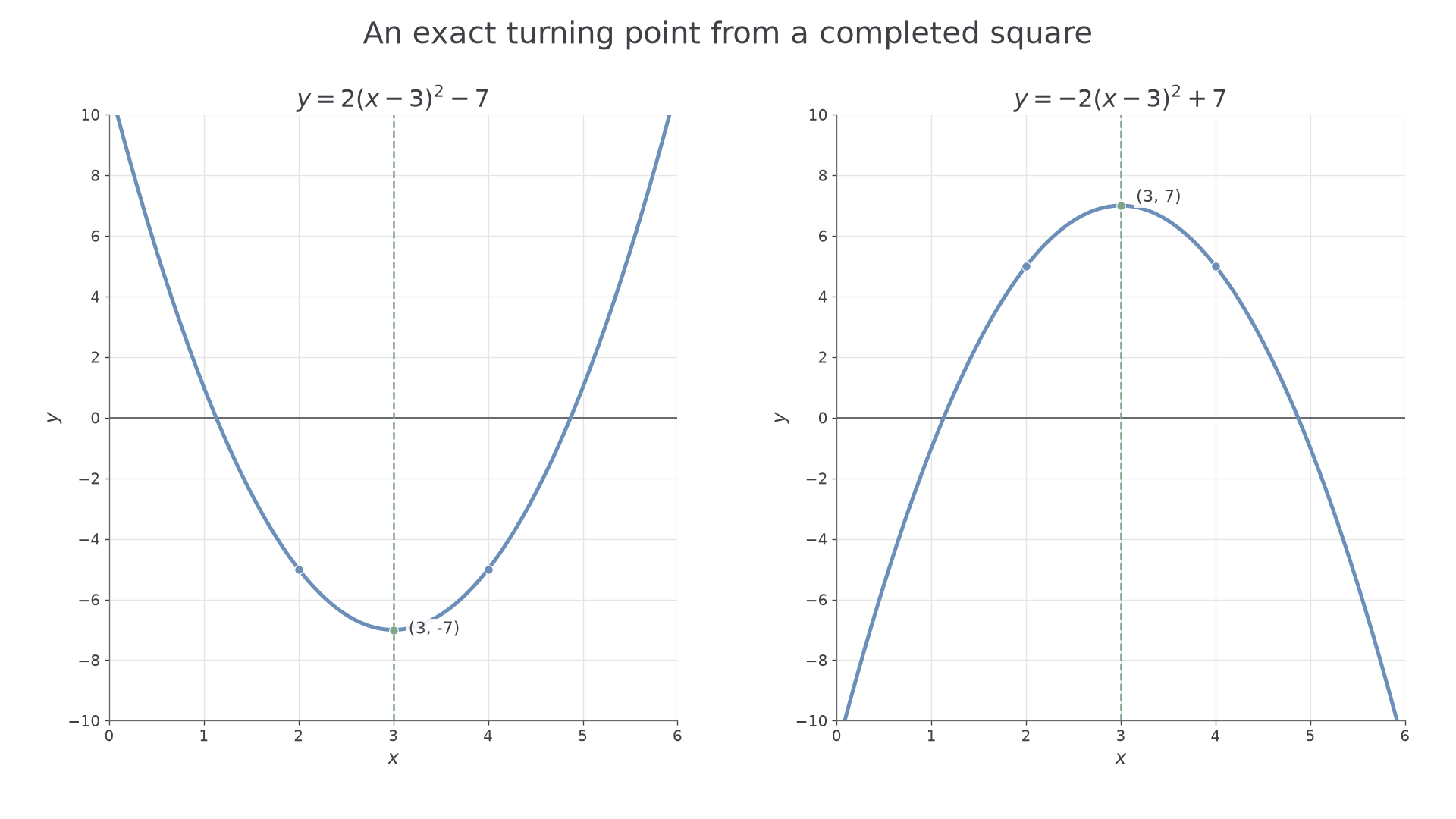
Worked example 1: a minimum with a non-unit coefficient
Question. Find the turning point of by completing the square. State whether it is a maximum or minimum.
Plan. Factor two from the first two terms, complete the square inside and use its least possible value.
Answer. The turning point is the minimum , with symmetry line .
Check. The original expression gives at . At the separate inputs 2 and 4, it gives both times, higher by 2 and equally spaced about the symmetry line.
Negate only the complete expression. The same squared bracket remains, but now non-zero squares lower the output.
Worked example 2: the corresponding maximum
Question. Find the turning point of by completing the square.
Plan. Factor out negative two, complete the same square and keep the inequality's meaning clear.
Answer. The turning point is the maximum , again on .
Check. Substitution into the original rule gives at 3. Inputs 2 and 4 both give 5, two lower. Expanding also returns the original quadratic.
You can now sketch a quadratic using its exact turning point as well as roots and intercepts. A minimum below the horizontal axis gives two crossings for an upward-opening full parabola; a minimum on it gives one distinct root; a minimum above it gives none. Reverse “below” and “above” for a downward-opening parabola with a maximum.
Watch out
In , the first coordinate is , not 2: solve . Also multiply the compensating constant by the outside coefficient when completing the square.
Reading exponential growth and decay
A quantity growing by 50% each hour adds different amounts each hour. Starting at 200 mg, it adds 100 mg in the first hour but 150 mg in the next. The repeated feature is the multiplier , not a fixed addition. That produces an exponential curve rather than a straight line.
Repeated proportional change
For an initial positive amount , a fixed multiplier per time unit gives
Growth by gives . Decay by , with , gives . In a continuous model, fractional describes times between whole units; a process updated only at whole times is represented by discrete points. Not given in the List of formulas: learn the multiplier method.
Choose the graph to match the model's time domain. Time since a start is normally , even though the algebraic expression can have values at negative inputs. Label the time unit and quantity unit; these are not interchangeable with the step number.
[DIAGRAM: asset_name: Equal percentage changes give curved graphs; asset_slug: growth_decay_models; caption: A fixed multiplier changes the amount added or lost at each step.; description: Two numbered grids plot mass in milligrams against time in hours from zero to four. One shows M equals two hundred times one point five to the t with points two hundred, three hundred, four hundred fifty, six hundred seventy-five and one thousand twelve point five. The other shows M equals two hundred times one half to the t with points two hundred, one hundred, fifty, twenty-five and twelve point five. Smooth curves represent the stated continuous models.]
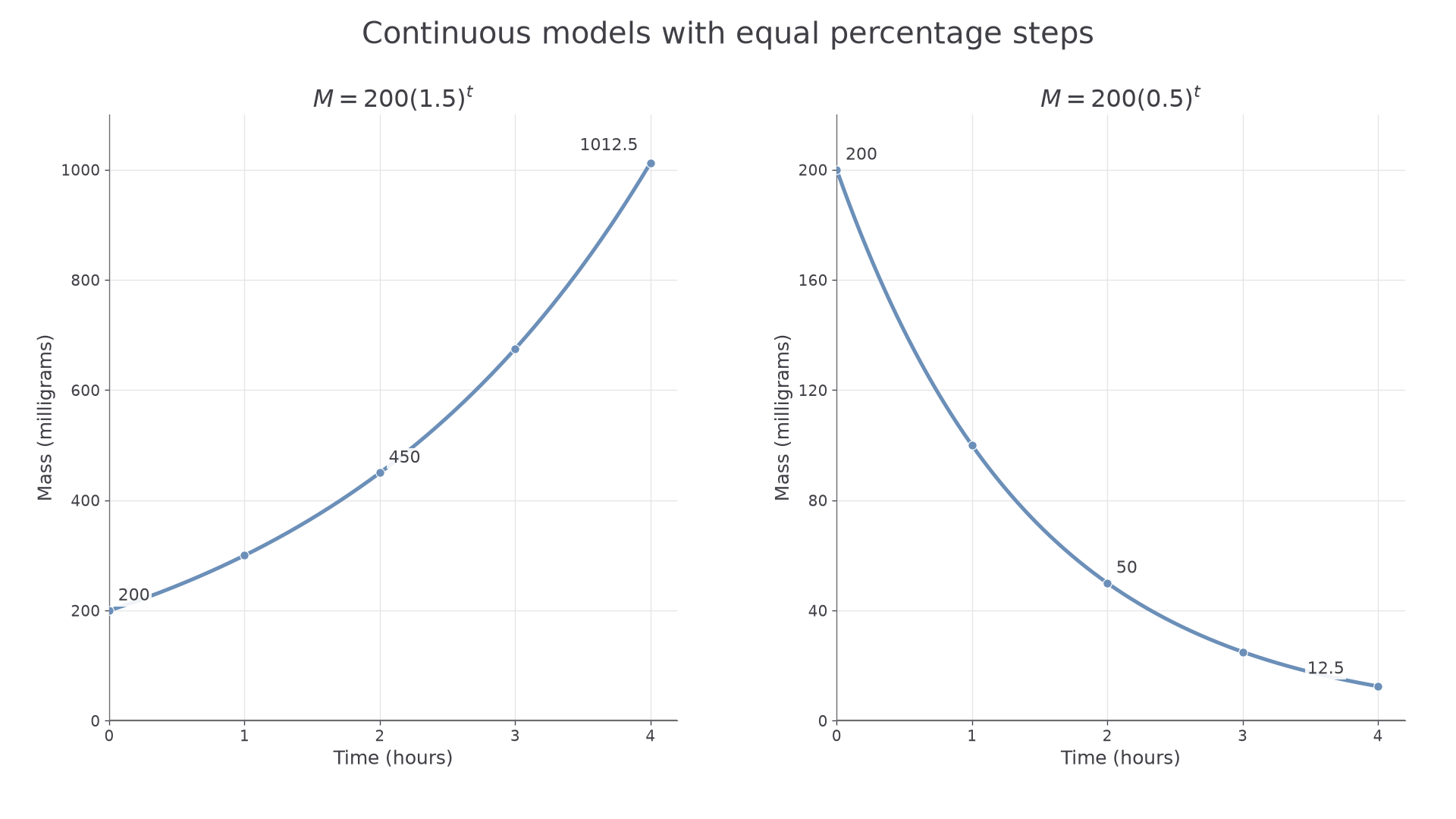
Worked example 3: 50% growth each hour
Question. A continuous culture-mass model is , with in milligrams and in hours after measurement begins. Calculate masses at , and describe the graph.
Plan. Multiply by 1.5 at each hour, and plot time horizontally.
Answer. The masses are mg. Draw the left increasing curve, becoming steeper as the amount added each hour increases.
Check. The successive differences are mg; each is half the preceding mass. Ratios of successive masses are all 1.5.
Continue this lesson.
You’re previewing NovaLearn without an account. Create a free account to read the rest.
Create free account