E2.10, E2.11 - Cubic, reciprocal and exponential curves
Different rules produce recognisable curve families, with different allowed inputs and long-term behaviour. You will build tables and draw the power and exponential graphs in E2.10, then recognise and sketch cubic, reciprocal and exponential forms for E2.11, using roots, symmetry and asymptotes.
Power and reciprocal curve families
How can a curve get closer and closer to a line without meeting it? The reciprocal curve already hints at the answer. Before studying its distant behaviour, check which inputs its rule allows: a graph cannot contain a point where its calculation is undefined.
The domain is the set of allowed inputs. A square root means the non-negative real root, so needs . A square root in a denominator needs : zero is now excluded too.
Power terms and domains
These power terms can be combined, with rational coefficients, in sums of at most three terms:
| Power | Equivalent expression | Allowed real inputs |
|---|---|---|
| constant term | all real inputs | |
| , , | linear, square, cube terms | all real inputs |
The exponent-zero term is written as a constant. There is no need to evaluate to use a constant function at zero. Every displayed denominator and square root must be defined. Simplifying an expression does not restore an input excluded by its original rule: even excludes zero.
[DIAGRAM: asset_name: Power shapes and their domains; asset_slug: power_domains; caption: A root in the denominator excludes zero as well as negative inputs.; description: Four numbered grids show y equals one over x squared with two positive branches and y-axis symmetry, y equals one over the square root of x on positive inputs only, y equals the square root of x beginning at the origin, and y equals one over x with opposite-sign branches. Each rule is labelled on its grid.]
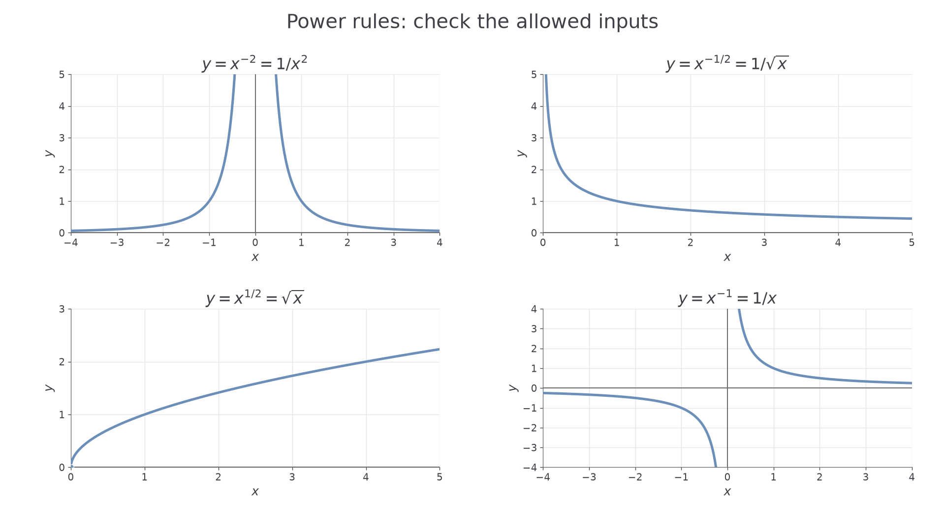
For example, is positive on both sides of zero and symmetric about the vertical axis; changes sign and has half-turn symmetry about the origin. Squaring and taking a reciprocal are different operations from taking a square root.
For compact substitution work, means “the output when ”. Similarly, for a mass model depending on time , means its mass at . These brackets identify an input; they do not mean multiplication.
Worked example 1: two power terms
Question. Make a table for at . State its domain.
Plan. Square each input before dividing, then add the linear term.
Answer. The outputs are . The domain is all real . Plot the two input ranges separately, as in the left graph below.
Check. At each calculated pair, . For , , checking the combined expression by undoing its operations.
Change only the negative exponent from to . The denominator is now a square root, so the allowed inputs change as well as the values.
Worked example 2: a root in the denominator
Question. Make the corresponding table for at . State its domain and find its output at .
Plan. Reject inputs without a real square root, then use the positive square root in the denominator.
Answer. No real outputs at ; outputs 5 and 9.5 at 1 and 4. At 9 the output is 19. The domain is , as in the right graph below.
Check. Undoing the operations gives . At , . Zero is excluded because its root would be the denominator zero.
[DIAGRAM: asset_name: Changing one exponent changes the domain; asset_slug: power_sum_tables; caption: The first rule allows negative inputs; the second has real values only to the right of zero.; description: Two numbered grids show y equals two x plus three over x squared, with separated negative-input and positive-input branches, and y equals two x plus three over square root x on positive inputs only. Calculated table points are marked. The second also marks nine comma nineteen.]
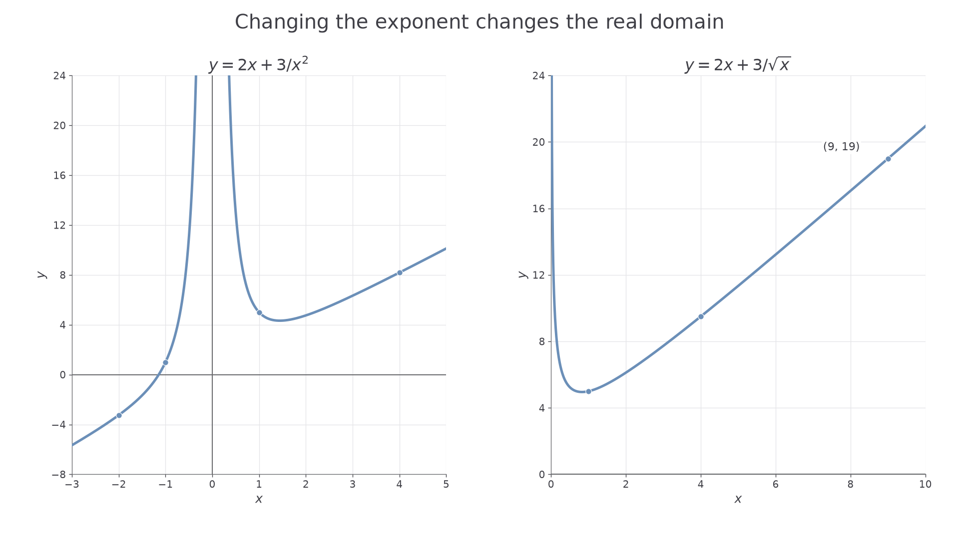
A graph solves equations for these families too. For example, reaches height 2.5 at ; squaring 2.5 checks the read input. Shifted reciprocals such as retain the excluded zero but move every output down by one. We will identify their limiting lines in the last part.
Watch out
means , not or . Rewrite a fractional negative power before substituting.
Cubic shapes and roots
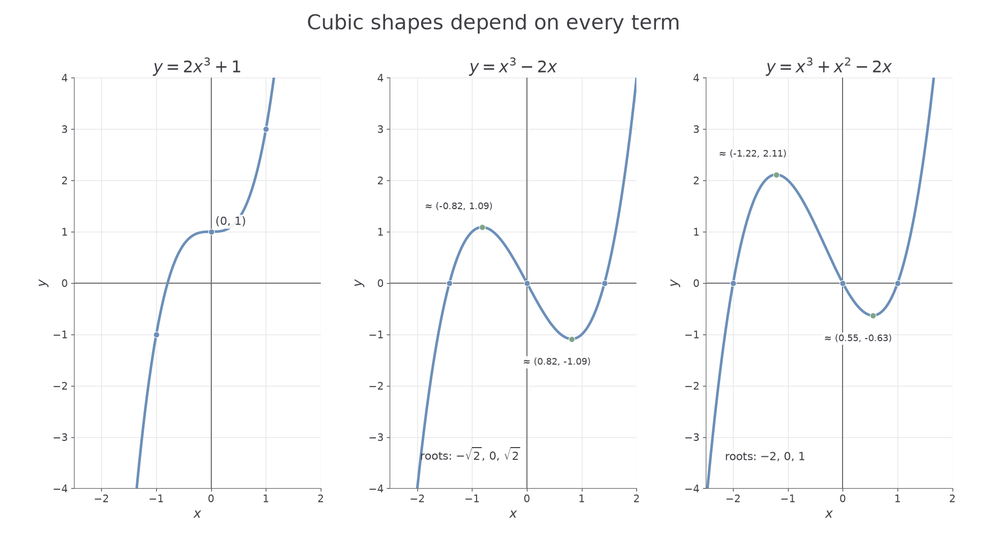
A cubic has highest non-zero power three. The simple family , with , has a rising S-shape when and a falling S-shape when . It has half-turn symmetry about , not mirror symmetry about the vertical axis. For instance, passes through , and ; a half-turn around swaps the outer points. Its real root is approximately .
Adding other powers can create a local highest point and a local lowest point, called turning points. A graph rises then falls at a local maximum, and falls then rises at a local minimum. “Local” compares nearby points: the whole cubic still continues beyond the displayed window. Here, estimate these coordinates graphically; no differentiation is needed.
[DIAGRAM: asset_name: Cubic shapes, roots and local turns; asset_slug: cubic_shapes; caption: Adding a squared term can move the roots and remove symmetry about the origin.; description: Three numbered coordinate grids show the simple cubic y equals two x cubed plus one, y equals x cubed minus two x, and y equals x cubed plus x squared minus two x. The middle graph has roots negative square root two, zero and square root two and approximate turns at negative zero point eight two comma one point zero nine and zero point eight two comma negative one point zero nine. The right has roots negative two, zero and one and approximate turns at negative one point two two comma two point one one and zero point five five comma negative zero point six three.]
Worked example 3: an origin-symmetric cubic
Question. Find the roots of , describe its symmetry and estimate its turning points from the middle graph.
Plan. Factor out for the zeros, compare opposite inputs and read the local changes of direction.
Answer. Roots ; half-turn symmetry about the origin. The local maximum is approximately , and the local minimum approximately .
Check. Substitution of gives . Also, and are a half-turn pair, and both lie near the corresponding graph turns. Their heights are not the exact local extremes.
Add only the squared term . This preserves a zero at the origin but changes the other roots and the symmetry.
Worked example 4: adding a squared term
Question. Find the roots of , and estimate its turning points from the right graph. Is it still symmetric about the origin?
Plan. Factor the expression, then test a pair of opposite inputs before accepting the earlier symmetry.
Answer. Roots . The local maximum is approximately , and local minimum approximately . It does not have half-turn symmetry about the origin.
Check. Direct substitution at gives , and at 1 gives . The nearby heights at and 0.6 are 2.112 and , consistent with the two estimated turns.
For accurate drawings, make a table over the requested interval and add points around close roots or changes of direction. For sketches, show the arm directions, intercepts and significant turns. A generic S with only one crossing would miss the three roots in each worked example. A cubic's symmetry need not be about the origin; do not infer that all possible symmetry is absent merely because the origin test fails.
Watch out
“Contains ” does not guarantee the simple shape. Lower powers can create two local turns and three distinct crossings. Read or calculate the features of the actual rule.
Continue this lesson.
You’re previewing NovaLearn without an account. Create a free account to read the rest.
Create free account