Xc1–Xc4 - Surfaces, partial derivatives and stationary points | OCR A-Level Further Mathematics B (MEI)

Xc1–Xc2 turn a function of two variables into a surface, vertical sections and horizontal contours. Xc3 introduces first-order partial derivatives. Xc4 uses them to locate stationary points, with any investigation of their nature guided by a supplied method.

Fixing one input cuts a surface into a curve

Can both coordinate sections through a point be perfectly flat, yet the point be neither a maximum nor a minimum? The surface $z=xy$ does exactly that at the origin. To see why, we first need to distinguish a surface from the curves cut out of it.

You already know

A graph $z=f(x)$ relates one input to one output. A point in three dimensions needs three ordered coordinates $(x,y,z)$ . Substituting a fixed value for one variable leaves an expression in the remaining variables.

For example, $z=x^2+2y^2$ assigns a height to each input pair. At $(x,y)=(1,2)$ , its height is $9$ , giving the surface point $(1,2,9)$ .

Surface and coordinate section

The graph $z=f(x,y)$ consists of all points $(x,y,f(x,y))$ for allowed pairs $(x,y)$ .

A section with $x=a$ is the curve $z=f(a,y)$ lying in the vertical plane $x=a$ . A section with $y=b$ is $z=f(x,b)$ , lying in the plane $y=b$ .

The fixed coordinate still matters when you locate the curve in space. A sketch in $(y,z)$ coordinates describes an $x=a$ section, but a point on the surface still needs its $x$ -coordinate.

Worked example 1: fix x

Question. For $z=x^2+2y^2$ , describe and sketch the section $x=1$ , giving its lowest point in three dimensions.

Plan. Substitute $x=1$ , then read the resulting parabola in the remaining variable.

\begin{aligned} z&=1+2y^2 && \text{section in the plane }x=1\\ z&\ge1 && y^2\ge0\\ y&=0,\quad z=1 && \text{vertex of the section} \end{aligned}

Why this step? The vertex $(y,z)=(0,1)$ in the section sketch corresponds to $(1,0,1)$ on the surface.

Answer. An upward-opening parabola in $x=1$ , with lowest point $(1,0,1)$ .

Check. The point $(1,1,3)$ satisfies both the surface and this section.

Change only which coordinate is fixed at $1$ : use $y=1$ instead.

Worked example 2: fix y

Question. Describe and sketch the section $y=1$ of the same surface.

Plan. Substitute $y=1$ , retaining $x$ as the varying coordinate.

\begin{aligned} z&=x^2+2 && \text{section in the plane }y=1\\ z&\ge2 && x^2\ge0\\ x&=0,\quad z=2 && \text{vertex} \end{aligned}

Why this step? Fixing $y$ is a different cut from fixing $x$ ; the coefficients of $x^2$ and $y^2$ need not agree.

Answer. An upward-opening parabola in $y=1$ , with lowest point $(0,1,2)$ .

Check. It also passes through $(1,1,3)$ , where the two section planes meet the surface.

[DIAGRAM: asset_name: Coordinate sections of an elliptic bowl; asset_slug: h645_b146_sections; caption: Fixing x or y produces a curve in the corresponding vertical plane; description: An exact three-dimensional plot of z equals x squared plus twice y squared highlights the x equals one section in clay and the y equals one section in sage. Two adjacent coordinate plots show z equals one plus twice y squared and z equals x squared plus two, with their vertices labelled. The common surface point one comma one comma three is marked.]
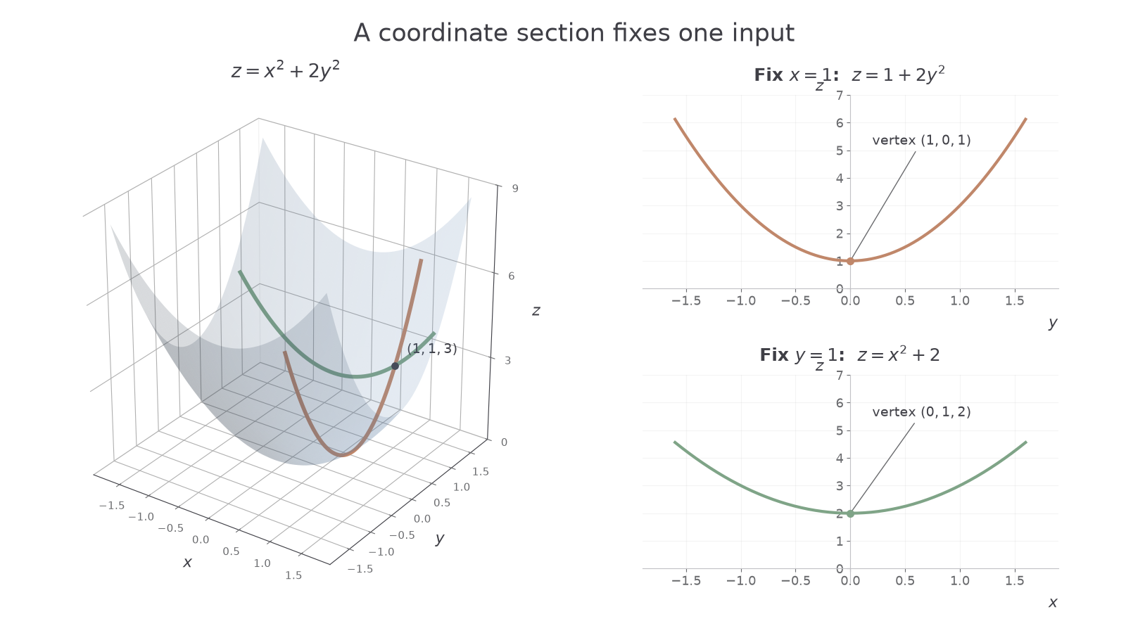
Fixing x or y produces a curve in the corresponding vertical plane

There is no extra section formula in the booklet: substitute the fixed coordinate into the given function. Label the correct remaining horizontal variable on a section sketch.

Watch out

Wrong: report $(0,2)$ as a point on a three-dimensional surface.

Right: retain the fixed coordinate. The vertex of the $y=1$ section is $(0,1,2)$ .

Move the fixed $y$ -coordinate to a new plane.

A contour fixes the height

A horizontal cut fixes $z$ , rather than $x$ or $y$ . For the bowl $z=x^2+2y^2$ , fixing $z=2$ gives $x^2+2y^2=2$ . Its projection onto the $xy$ -plane is an ellipse; the actual contour lies at height $2$ .

Contour

A contour at height $c$ consists of the surface points satisfying $f(x,y)=c$ , with $z=c$ . A contour plot draws the corresponding curves in the $xy$ -plane and labels each with its height.

For example, a vertical section fixes an input coordinate; a contour fixes the output.

A contour need not be a closed curve. Depending on the function and height, it can be a hyperbola, several pieces, a single point or empty.

Worked example 3: an elliptical contour

Question. Sketch the contour $z=2$ on $z=x^2+2y^2$ , giving its intercepts as surface points.

Plan. Fix the height and put the resulting equation into standard ellipse form.

\begin{aligned} x^2+2y^2&=2 && \text{fixed surface height}\\ \frac{x^2}{2}+y^2&=1 && \text{ellipse in the }xy\text{-plane}\\ y=0&\implies x=\pm\sqrt2 && \text{x-intercepts}\\ x=0&\implies y=\pm1 && \text{y-intercepts} \end{aligned}

Why this step? The ellipse equation describes the plan view, while the height $z=2$ locates the contour in space.

Answer. An ellipse with surface intercepts $(\pm\sqrt2,0,2)$ and $(0,\pm1,2)$ .

Check. Every intercept gives $x^2+2y^2=2$ . For this bowl, height $0$ gives just the origin; negative heights give no contour.

Keep the height $2$ , but change the surface to $z=xy$ .

Worked example 4: a hyperbolic contour

Question. Sketch the contour $z=2$ on $z=xy$ .

Plan. Solve the fixed-height relation for $y$ and identify its branches.

\begin{aligned} xy&=2 && \text{fixed height}\\ y&=\frac2x,\quad x\ne0 && \text{plan-view curve}\\ x>0&\implies y>0,\qquad x<0\implies y<0 && \text{branch locations} \end{aligned}

Why this step? A positive product requires matching signs. The coordinate axes are asymptotes, not parts of this non-zero contour.

Answer. A rectangular hyperbola in the first and third quadrants, lying at height $2$ on the surface.

Check. $(1,2,2)$ and $(-1,-2,2)$ are on it. At height $0$ , the relation instead becomes the union of the two coordinate axes.

[DIAGRAM: asset_name: Different surfaces give different contour patterns; asset_slug: h645_b146_contours; caption: A contour label gives the height, while the drawn coordinates are x and y; description: One panel shows ellipses x squared plus twice y squared equals two, eight and eighteen, with those height labels. A second panel shows xy equals two in the first and third quadrants and xy equals minus three in the second and fourth quadrants. Coordinate axes are labelled and contour branches remain separated from their asymptotes.]
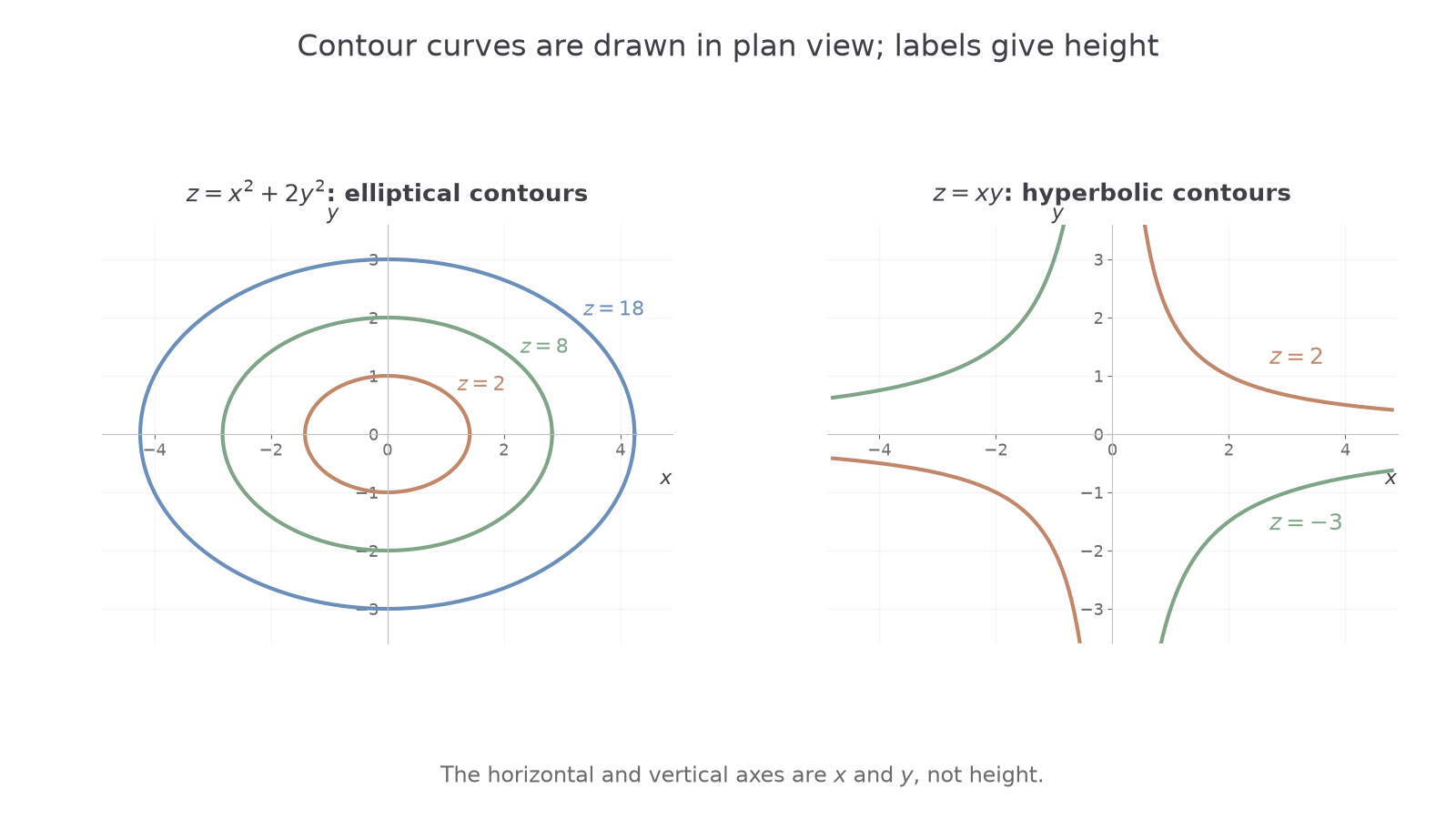
A contour label gives the height, while the drawn coordinates are x and y

These contour equations come from substitution, not a separate booklet formula. To sketch a useful contour, mark its level, intercepts where they exist, branch locations and any asymptotes.

Watch out

Wrong: call $x=1$ a contour because one coordinate has been fixed.

Right: $x=1$ gives a vertical section. A contour fixes $z$ .

Change only the hyperbola's contour height.

Differentiate with the other input held constant

The slope of a surface depends on the direction in which you move. Holding $y$ fixed gives a section in which $x$ varies; its slope is the partial derivative with respect to $x$ . Holding $x$ fixed gives the other coordinate slope.

First-order partial derivative

For $z=f(x,y)$ , $\partial z/\partial x$ differentiates with respect to $x$ while treating $y$ as constant. Likewise, $\partial z/\partial y$ treats $x$ as constant.

For example, $\partial(xy^2)/\partial x=y^2$ , while $\partial(xy^2)/\partial y=2xy$ .

Use the ordinary differentiation rules, including product and chain rules, with the other input fixed. A constant with respect to one variable can still be an expression in the other variable.

Worked example 5: two coordinate slopes

Question. Find the first-order partial derivatives of $z=x^2y+3xy^2-4x$ , and evaluate them at $(x,y)=(1,2)$ .

Plan. Differentiate one input at a time, then substitute the point.

\begin{aligned} \frac{\partial z}{\partial x}&=2xy+3y^2-4 && y\text{ held constant}\\ \frac{\partial z}{\partial y}&=x^2+6xy && x\text{ held constant}\\ \left.\frac{\partial z}{\partial x}\right|_{(1,2)}&=4+12-4=12 && \text{x-direction slope}\\ \left.\frac{\partial z}{\partial y}\right|_{(1,2)}&=1+12=13 && \text{y-direction slope} \end{aligned}

Why this step? In the first derivative, $3y^2$ is the coefficient of $x$ ; in the second, $3x$ is the coefficient of $y^2$ .

Answer. The partial derivatives are $2xy+3y^2-4$ and $x^2+6xy$ , giving slopes $12,13$ .

Check. The fixed- $y=2$ section is $z=2x^2+8x$ , whose slope at $x=1$ is $12$ .

Continue this lesson.

You’re previewing NovaLearn without an account. Create a free account to read the rest.

Create free account

Last Accessed

Core Pure

Mechanics (Major and Minor)

Statistics (Major and Minor)

Modelling with Algorithms

Numerical Methods

Extra Pure

Further Pure with Technology

Xc1–Xc4 - Surfaces, partial derivatives and stationary points

Fixing one input cuts a surface into a curve

A contour fixes the height

Differentiate with the other input held constant

Continue this lesson.

Learn faster with Nova