SR27–SR29 - Combining Normal random variables
SR27 extends expectation algebra to continuous variables. SR28 uses calculator probabilities and percentiles for a Normal model; SR29 adds the crucial distribution result for independent Normal combinations. You will state the resulting distribution before calculating a probability, and distinguish fresh observations from multiples of one variable.
Specify the Normal model before using the calculator
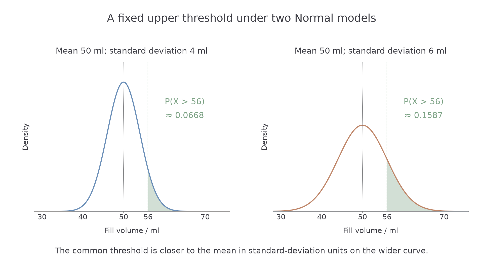
A dispenser has mean fill and standard deviation . If a second dispenser has the same mean but a larger standard deviation, will more of its fills exceed ?
A wider Normal curve spreads probability further from its centre. The threshold stays fixed, but its distance in standard deviations changes. A sketch tells you which tail to calculate before you press a key.
Normal distribution
The notation , with , describes a continuous Normal model with mean , variance and standard deviation . Its density is a symmetric bell-shaped curve centred at , with total area one.
For example, has standard deviation , not . The full mathematical model has unbounded support; judge its suitability for a physical measurement in context.
Use the calculator's Normal probability or inverse Normal function. Enter the standard deviation if that is what the calculator requests, even though distribution notation gives the variance. An inverse Normal input is a cumulative probability to the left.
[DIAGRAM: asset_name: The same threshold under two Normal models; asset_slug: h645_b100_normal_tails; caption: With the same mean, a greater standard deviation puts more probability above this fixed upper threshold; description: Two panels show Normal curves with mean fifty and standard deviations four and six. The region to the right of fifty six is shaded sage in each. The tails are labelled approximately 0.0668 and 0.1587, and the common mean and threshold are marked without using the formula for a Normal pdf.]
Worked example 1: an upper tail and a percentile
Question. Fill volume , in millilitres, is modelled by . Find and the volume below which of fills lie.
Plan. Use an upper-tail Normal calculation, then invert cumulative probability , with mean and standard deviation .
Why this step? The upper tail uses probability above the threshold, whereas inverse Normal uses the left-hand probability up to the unknown value.
Answer. to decimal places; the 90th percentile is to significant figures.
Check. is standard deviations above the mean, so a small upper tail is sensible. The 90th percentile is below , because more than lie below .
Change only the standard deviation from to , keeping the mean and threshold fixed.
Worked example 2: more spread, more upper-tail probability
Question. Repeat the probability and percentile calculations for .
Plan. Use the same statistical functions with standard deviation .
Why this step? The threshold is now only one standard deviation above the mean, rather than . The tail must be larger.
Answer. Probability , and 90th percentile .
Check. The new percentile is further above , and now exceeds , consistent with a tail above greater than .
No Normal density integration is needed. The model, requested event and calculator parameters should be visible in your working. The inverse-probability procedure is not a separately printed formula in the booklet; the booklet provides selected standard Normal percentage points, while these calculations use statistical calculator functions.
Watch out
Wrong: enter as the standard deviation for . Right: its variance is , so enter standard deviation . Check the calculator's parameter labels.
Now reduce only the standard deviation.
A Normal combination needs the right assumptions
The expectation and variance rules already used for discrete variables also apply to continuous variables with the required finite moments. The new conclusion is about shape: a linear combination of mutually independent Normal variables is itself Normal.
You already know
Expectation uses signed coefficients and does not require independence. Variance of an independent combination adds squared-coefficient contributions; constants add no variance. The same variable repeated is not a fresh independent observation.
First identify each random quantity and its coefficient. Then state the distribution of the combination, not just its mean and variance.
Independent Normal combinations
If and are independent, then
The same result extends to more mutually independent Normal variables. A single linear transformation is Normal too, provided its scale factor is non-zero. A zero total variance instead gives a constant.
Not in the formula booklet: learn it.
Use the result without proving it. Knowing only a mean and variance does not establish a Normal shape; for example, a sum of two uniform variables is not generally Normal. Independence is also needed for the displayed variance rule.
Worked example 3: a difference of Normal contributions
Question. Independent variables have distributions and . Let . Find the distribution of , and hence .
Plan. Combine the means and variances, retain Normality, then calculate the tail.
Why this step? Subtracting changes the mean's sign contribution, but its variance contribution remains positive.
Answer. , with .
Check. The threshold is one standard deviation above the new mean , matching the familiar upper tail from the preceding part.
Continue this lesson.
You’re previewing NovaLearn without an account. Create a free account to read the rest.
Create free account