SR19–SR21 - Probability density functions
SR19–SR21 model measurements using continuous random variables. You will interpret a density graph, check that a proposed density is valid, sketch its support and calculate probabilities as areas, including when the formula changes partway through an interval.
A density height can exceed one
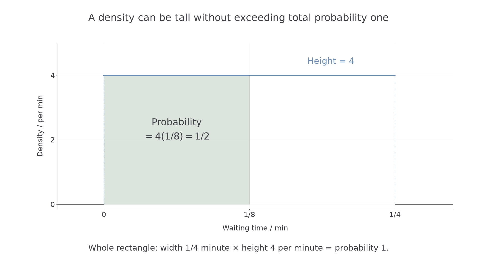
A waiting time is equally likely to fall anywhere in a quarter-minute interval. Its density graph has height . Has somebody invented a probability greater than one?
The graph is a rectangle of width minute and height per minute. Its total area is . Half the interval has area , whatever the height of the rectangle. Area, rather than height, is the probability.
You already know
Probabilities lie between and , and the total probability is . Integration finds area under a non-negative curve. A measurement such as time is modelled differently from an integer count.
A continuous model allows all real values in an interval. Recorded measurements may be rounded, but the model describes the underlying quantity before rounding.
Probability density function
A probability density function, or pdf, , describes how the probability of a continuous random variable is distributed. The probability in an interval is the area under its graph over that interval.
The support is the region on which values can occur; always specify the density outside it, usually as zero. A waiting time can be continuous; the number of customers waiting is discrete.
For a continuous variable, a single point has zero width and hence zero probability: . Thus changing an interval endpoint from strict to inclusive does not change its probability. A density height is not , and a zero-probability exact value is not logically impossible.
[DIAGRAM: asset_name: A tall uniform density with total area one; asset_slug: h645_b097_tall_density; caption: Density height four is valid because the rectangle has width one quarter and area one; description: A density graph is zero outside the interval from zero to one quarter. Within it a rectangle has height four. Its left half, ending at one eighth, is shaded sage and labelled probability one half. The vertical axis is density per minute and the horizontal axis is waiting time in minutes.]
Key idea
A pdf is a density of probability per unit of the variable. Its height may exceed ; its total area must equal .
A continuous uniform, also called rectangular, model suits a value equally likely to fall in equal-length subintervals. A Normal model can suit a roughly symmetric cluster of measurements. Other shapes may fit other situations; use a supplied density rather than assuming every continuous measurement is uniform or Normal.
Check non-negativity and total area
A proposed pdf needs two checks: it must never be negative, and its area must be one. Neither check replaces the other.
For example, on cannot be a pdf because it is negative on part of its stated support. Solving an area equation cannot rescue a negative density.
A valid pdf and interval probabilities
A pdf satisfies
For a pdf supported on a finite interval ,
and, for ,
These are properties of a continuous probability model. The booklet's cdf integral expresses the same area principle, but these conditions and interval form are not printed separately.
Not in the formula booklet: learn it.
Show the relevant definite integral before evaluating it, even if you then use a calculator. A sketch should show the support, important heights, the shape and zero density elsewhere. The density may jump at a boundary; it need not join the zero branch continuously.
Worked example 1: normalising a decreasing density
Question. A proposed pdf is
Find , justify that the resulting pdf is valid and describe its sketch.
Plan. Set the total area to one, then check the sign and endpoints.
Why this step? The area determines , but validity also needs throughout the stated interval.
Answer. . The density is non-negative and has total area one. Its sketch is a straight line from to , with zero density outside .
Check. The triangular area is .
Change only the intercept in the unnormalised expression, from to . The line no longer reaches zero at the right endpoint, so its area is a trapezium.
Continue this lesson.
You’re previewing NovaLearn without an account. Create a free account to read the rest.
Create free account