Tc9, Tc10 - Runge-Kutta methods | OCR A-Level Further Mathematics B (MEI)

Use four-stage Runge–Kutta calculations and implement them in a spreadsheet. You will explain the stage points and weights, adapt the differential equation and step length, and read a supplied variation carefully rather than force every method into the standard pattern.

Four trial gradients make one corrected step

Could four gradient readings land exactly on a curved solution after one large step?

Sometimes they can. For $y'=3x^2$ , $y(0)=1$ , the standard four-stage method with $h=1$ gives exactly $y(1)=2$ , matching $y=x^3+1$ . That special success is useful to understand, but it is not a promise of exactness for every differential equation.

You already know

Modified Euler samples a starting gradient and a predicted endpoint gradient, then combines their increments. Each increment already contains the step length. A predicted stage point is an aid to the calculation, not a new confirmed point on the solution curve.

The standard fourth-order Runge–Kutta method uses the start, two different midpoint predictions and one endpoint prediction. Each new stage uses information from the preceding stage.

Standard fourth-order Runge–Kutta method

For $y'=f(x,y)$ , starting from $(x_n,y_n)$ ,

\begin{aligned} k_1&=h f(x_n,y_n)\\ k_2&=h f\left(x_n+\frac h2,y_n+\frac{k_1}{2}\right)\\ k_3&=h f\left(x_n+\frac h2,y_n+\frac{k_2}{2}\right)\\ k_4&=h f(x_n+h,y_n+k_3)\\ x_{n+1}&=x_n+h\\ y_{n+1}&=y_n+\frac{k_1+2k_2+2k_3+k_4}{6} \end{aligned}

All four evaluations must be defined. The $k_i$ are increments; there is no extra multiplication by $h$ in the final weighted average.

In the formula booklet.

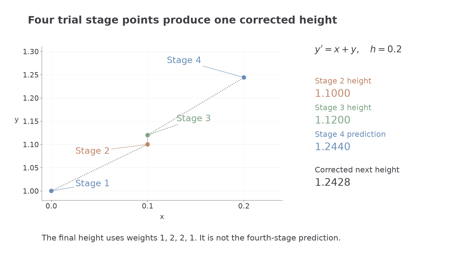
The two midpoint stages have the same $x$ -coordinate but generally different predicted $y$ -coordinates. Their doubled weights do not mean that the method takes two actual half steps.

Worked example 1: one four-stage step

Question. For $y'=x+y$ , $y(0)=1$ , calculate one standard Runge–Kutta step with $h=0.2$ .

Plan. Calculate the increments in order, then combine them with weights $1,2,2,1$ .

\begin{aligned} k_1&=0.2(0+1)=0.2 && \text{starting point}\\ k_2&=0.2(0.1+1.1)=0.24 && \text{first midpoint prediction}\\ k_3&=0.2(0.1+1.12)=0.244 && \text{revised midpoint prediction}\\ k_4&=0.2(0.2+1.244)=0.2888 && \text{endpoint prediction}\\ y_1&=1+\frac{0.2+2(0.24)+2(0.244)+0.2888}{6} =1.2428 && \text{weighted correction} \end{aligned}

Why this step? The second midpoint height uses $k_2/2=0.12$ , rather than reusing $k_1/2=0.1$ .

Answer. $y(0.2)\approx1.2428$ from this single step.

Check. The analytical solution $y=2e^x-x-1$ gives $y(0.2)=1.24280552\ldots$ , close to the numerical estimate but not identical.

Change only $h$ to $0.1$ , leaving the equation and starting point unchanged.

Worked example 2: halve the one-step interval

Question. Calculate one standard Runge–Kutta step with $h=0.1$ .

Plan. Recalculate every stage with the new step, rather than halve the earlier increments.

\begin{aligned} k_1&=0.1(0+1)=0.1 && \text{new starting increment}\\ k_2&=0.1(0.05+1.05)=0.11 && \text{new midpoint}\\ k_3&=0.1(0.05+1.055)=0.1105 && \text{revised midpoint}\\ k_4&=0.1(0.1+1.1105)=0.12105 && \text{new endpoint prediction}\\ y_1&=1+\frac{0.1+2(0.11)+2(0.1105)+0.12105}{6} =1.110341666\ldots && \text{weighted correction} \end{aligned}

Why this step? A changed step changes both coordinates of the stage points, so the increments are not simply scaled copies.

Answer. $y(0.1)\approx1.11034167$ . One step now reaches $0.1$ , not $0.2$ .

Check. The exact value is $1.11034184\ldots$ . To compare methods at $x=0.2$ , take a second $0.1$ step instead of comparing these different endpoints directly.

For the opening equation $y'=3x^2$ , the four increments are $0,0.75,0.75,3$ . Their weighted combination is

\frac{0+2(0.75)+2(0.75)+3}{6}=1

so $y_1=2$ , exactly as claimed. The right side depends only on $x$ , so the trial heights do not affect these particular readings. The exact result is a feature of this equation, not a general error rule.

[DIAGRAM: asset_name: Four Runge-Kutta stage points; asset_slug: rk4_stage_points; caption: Two midpoint predictions share x but need not share y; description: A schematic mathematical stage plot for y'=x+y, h=0.2, starting at (0,1), labels stage 1 at (0,1), stage 2 at (0.1,1.1), stage 3 at (0.1,1.12), stage 4 at (0.2,1.244). The final corrected point (0.2,1.2428) is shown separately using a magnified inset or a side table so it is not confused with the predicted endpoint. A note gives weights 1,2,2,1.]
Two midpoint predictions share x but need not share y

Watch out

Wrong: set $k_3=k_2$ because both use the midpoint, or use $y_n+k_4$ as the next height. Right: use the distinct predicted heights and combine all four increments with the stated weights.

Apply the standard rule to one new step.

Make each stage a visible spreadsheet column

A spreadsheet makes a long chain of four-stage steps manageable. It must still show enough formulae to reveal the design: the starting conditions, parameter references, each stage and the next-row update.

Consider the family

y'=x-y+ay^2,\qquad y(0)=1

Store $h$ in $\text{J1}$ and $a$ in $\text{J2}$ . Set $\text{A2}=0$ , $\text{B2}=1$ , and use columns $\text{C:F}$ for the increments. Three auxiliary cells in $\text{G:I}$ hold the trial heights, keeping the formulae short. These literal entries use repeated multiplication for the square.

Cell	Formula
$\text{C2}$	$=\text{\$ J$1}(\text{A2}-\text{B2}+\text{$J$2}\text{B2}*\text{B2})$
$\text{G2}$	$=\text{B2}+\text{C2}/2$
$\text{D2}$	$=\text{\$ J$1}((\text{A2}+\text{$J$1}/2)-\text{G2}+\text{$J$2}\text{G2}*\text{G2})$
$\text{H2}$	$=\text{B2}+\text{D2}/2$
$\text{E2}$	$=\text{\$ J$1}((\text{A2}+\text{$J$1}/2)-\text{H2}+\text{$J$2}\text{H2}*\text{H2})$
$\text{I2}$	$=\text{B2}+\text{E2}$
$\text{F2}$	$=\text{\$ J$1}((\text{A2}+\text{$J$1})-\text{I2}+\text{$J$2}\text{I2}*\text{I2})$
$\text{A3}$	$=\text{A2}+\text{\$ J$1}$
$\text{B3}$	$=\text{B2}+(\text{C2}+2\text{D2}+2\text{E2}+\text{F2})/6$

Copy $\text{C2:I2}$ down, and copy $\text{A3:B3}$ down. Keep full stored precision. The stage formulae are applications of the supplied standard rule, not extra formulae to memorise; this worksheet layout is not printed in the booklet.

Worked example 3: check the spreadsheet against an analytical case

Question. Set $a=0$ , $h=0.1$ . Use the spreadsheet to estimate $y(0.4)$ .

Plan. Recalculate the four stages at each row, take four complete steps and compare with the analytical solution of $y'=x-y$ .

\begin{aligned} k_1&=0.1(0-1)=-0.1 && \text{first row}\\ k_2&=0.1(0.05-0.95)=-0.09 && \text{first midpoint}\\ k_3&=0.1(0.05-0.955)=-0.0905 && \text{revised midpoint}\\ k_4&=0.1(0.1-0.9095)=-0.08095 && \text{endpoint prediction}\\ y_1&=1+\frac{-0.1+2(-0.09)+2(-0.0905)-0.08095}{6} =0.909675 && \text{corrected value} \end{aligned}

$x_n$	Displayed $y_n$ , $8$ d.p.
$0.1$	$0.90967500$
$0.2$	$0.83746180$
$0.3$	$0.78163684$
$0.4$	$0.74064058$

Why this step? A known analytical case checks the worksheet before an equation without a convenient exact answer is investigated.

Answer. The estimate is $0.74064058$ , or $0.7406$ to $4$ decimal places.

Check. $y=2e^{-x}+x-1$ gives $y(0.4)=0.74064009\ldots$ , confirming this rounded result.

Continue this lesson.

You’re previewing NovaLearn without an account. Create a free account to read the rest.

Create free account

Last Accessed

Core Pure

Mechanics (Major and Minor)

Statistics (Major and Minor)

Modelling with Algorithms

Numerical Methods

Extra Pure

Further Pure with Technology

Tc9, Tc10 - Runge-Kutta methods

Four trial gradients make one corrected step

Make each stage a visible spreadsheet column

Continue this lesson.

Learn faster with Nova