Sb11, Sb12 - Regression on a non-random variable
Fit and use a least squares line when an experimenter controls the input and measures a variable response. Calculate residuals, judge a linear model informally and keep predictions within the role and range the model supports.
A controlled input and a random response
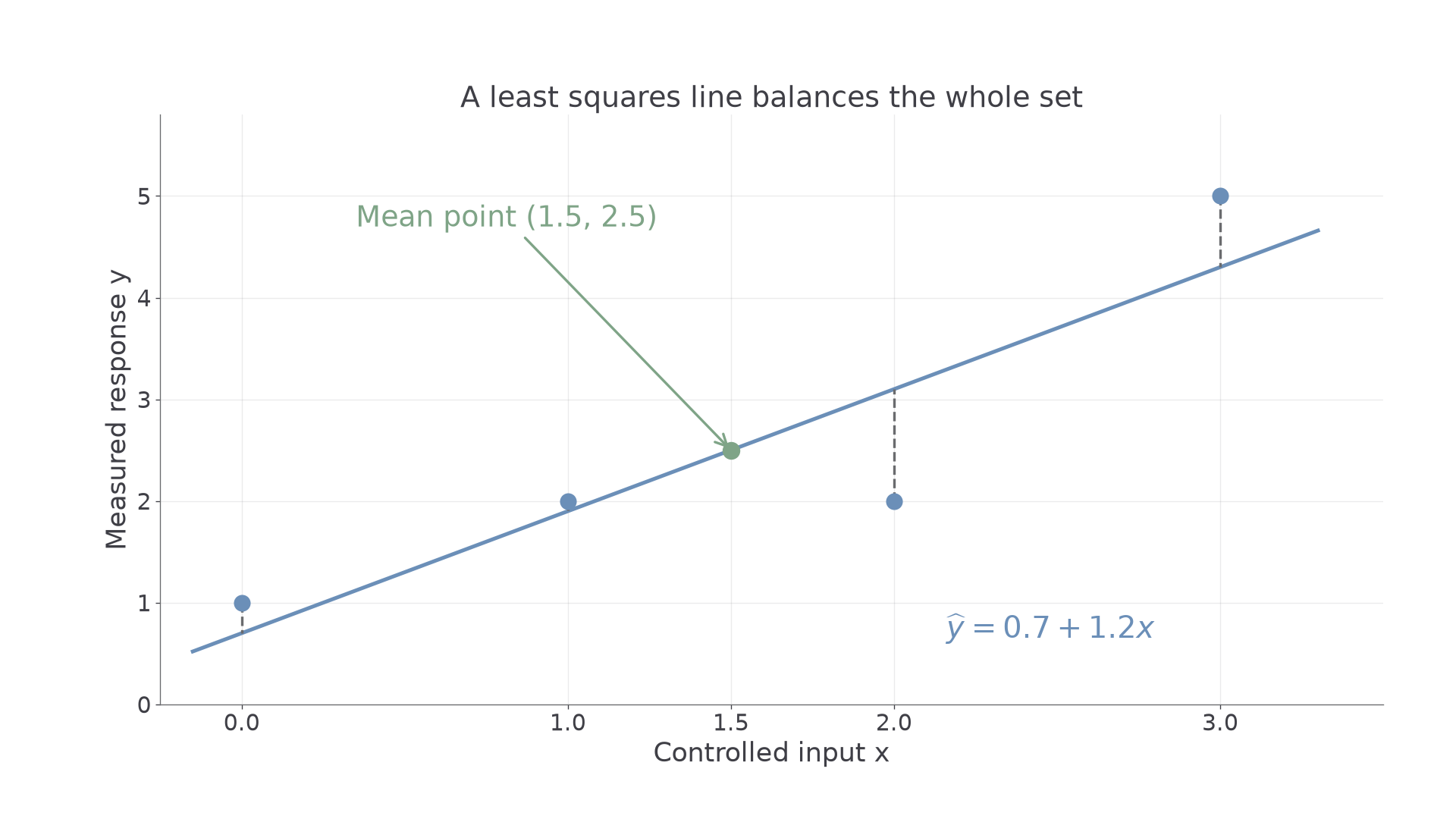
How can a best-fit line miss every observed point yet pass exactly through the point formed from the two means?
The line balances the observations as a group. It is not an instruction to join measured points, and it need not contain any individual observation.
You already know
Plot a controlled independent variable horizontally and its measured response vertically. Random-on-non-random data differ from two measurements that both vary across randomly sampled individuals.
Suppose an experimenter fixes a sensor's input level . Repeated measurements at that level can give different responses , owing to measurement variation or other uncontrolled influences. The input itself is treated as known, with negligible measurement error.
Regression of a response on a controlled input
A regression model for random on non-random uses fixed input values to estimate the underlying “true” response. Here that response is modelled as a linear function of the input; observations vary around it.
On a scatter diagram, repeated measurements at the same input lie on the same vertical line. Calculating the fitted line does not require the Pearson population-correlation test, which is inappropriate for this controlled-input setting.
Key idea
The model predicts the response at a chosen input. The controlled input is not another random response to be predicted by reversing the line.
Identify the model's direction.
Finding the least squares line
The least squares line minimises the sum of squared vertical differences between observed responses and fitted values. Large vertical discrepancies therefore count more than small ones. You need to use the fitted-line formula, not derive it.
Least squares regression of y on x
Write the fitted value as . Then
Equivalently,
The centred sums are
The input values must not all be identical.
In the formula booklet.
For raw data, a paired-variable calculator fit is expected: identify its coefficient convention rather than assuming that every calculator uses the same letters for intercept and gradient. For summary statistics, show your substitution.
Worked example 1: a calculator fit checked from totals
Question. Four fixed input levels and measured sensor responses, in appropriate units, are:
Find the least squares line for response on input.
Plan. Fit the paired data, then check gradient and intercept with the centred sums and means.
Why this step? We minimise vertical response errors, so the denominator is the input sum , not a response sum.
Answer. .
Check. At , the line gives .
Change only the last response, from to , and express the changed data through summaries.
Worked example 2: one observation changes
Question. The changed data have
Find the new regression line of response on input.
Plan. Recalculate the response mean and cross-product sum, retaining the unchanged input variation.
Why this step? Changing one response affects both its mean and its cross-products. Keeping the old intercept would leave the new line missing the new mean point.
Answer. .
Check. At , the predicted value is , the new response mean.
The opening puzzle now has its exact answer. The original line misses all four observed points but passes through . Every least squares line with an intercept passes through its mean point.
[DIAGRAM: asset_name: A fitted line passes through the means; asset_slug: controlled_regression_mean; caption: The original fitted line misses all four observations but passes through their mean point; description: The four blue observations (0,1), (1,2), (2,2), (3,5) are plotted with input x horizontally and response y vertically. The blue line y equals 0.7 plus 1.2x passes through a sage mean point at (1.5,2.5). Short vertical grey segments show the differences between each observation and the line. The mean point is labelled separately and no horizontal-distance minimisation is implied.]
Watch out
Wrong: reuse or totals from observations that were removed or corrected. Right: make sure every summary describes the same final set of pairs before fitting.
Change the last response once more.
Estimating in the appropriate direction and range
A fitted response is an estimate of the underlying response at an input, not a promise that the next observation will equal it.
Interpolation and extrapolation
Interpolation uses an input within the observed input range. Extrapolation uses one outside it. Extrapolation is more doubtful because the fitted linear relationship may not continue beyond the observed conditions.
Continue this lesson.
You’re previewing NovaLearn without an account. Create a free account to read the rest.
Create free account