SZ1, SZ2 - Simulating random variables | OCR A-Level Further Mathematics B (MEI)

Turn spreadsheet random numbers into discrete uniform, continuous uniform and Normal variables. You will build repeated trials, estimate probabilities and distributions from their output, and distinguish simulation variation from a faulty probability model.

From random decimals to equally likely integers

A spreadsheet's random-number function returns a decimal between $0$ and $1$ . How can it roll a fair die when its output is almost never a whole-number die score?

Split its interval into six equal pieces, and give every piece a die score. The lengths of the pieces, rather than the number of decimal places displayed, determine the probabilities.

You already know

A discrete uniform variable gives equal probability to each of its specified values. A continuous uniform variable gives probabilities proportional to interval lengths. Independent trials require fresh independent random inputs.

Write $U$ for a modelled continuous uniform random number on $[0,1]$ . A spreadsheet's $\operatorname{RAND}()$ provides a finite-precision version with $0\le U<1$ . The missing upper endpoint has probability zero in the ideal continuous model.

[DIAGRAM: asset_name: Equal intervals generate fair die scores; asset_slug: uniform_integer_mapping; caption: Six equal input intervals give six equally likely scores; description: A horizontal interval from 0 to 1 is divided at exact sixths into six equal bands labelled die scores 1 to 6. A clay marker at U=0.79 falls in the fifth band, so its simulated die score is 5. Boundary labels use half-open intervals, with each boundary assigned to the band on its right.]
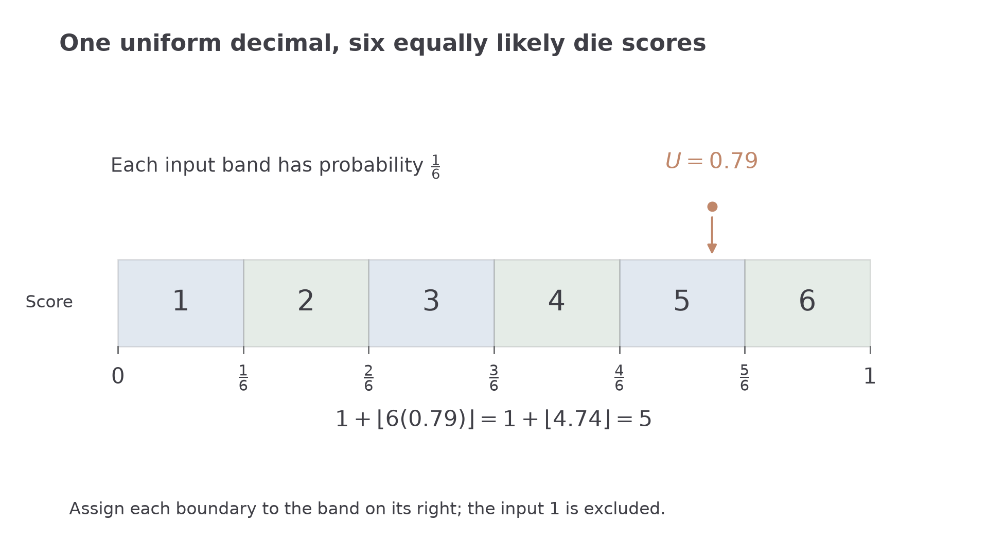
Six equal input intervals give six equally likely scores

Discrete uniform mapping

For integers $L\le H$ , let $m=H-L+1$ . Then

D=L+\lfloor mU\rfloor,\qquad 0\le U<1

is uniform on $\{L,L+1,\ldots,H\}$ . The floor $\lfloor z\rfloor$ is the greatest integer not exceeding $z$ . For non-negative inputs, the spreadsheet function $\operatorname{INT}$ performs this step.

Not in the formula booklet: learn it.

For a die, the intervals are $[0,1/6),[1/6,2/6),\ldots,[5/6,1)$ . Each has probability $1/6$ . In a spreadsheet, put $=\operatorname{RAND}()$ in cell $\text{A2}$ , then $=1+\operatorname{INT}(6*\text{A2})$ in $\text{B2}$ , and fill down. Within a spreadsheet formula, $*$ means multiplication.

Worked example 1: simulate a fair die

Question. Use $U=0.08,0.36,0.79,0.99$ to simulate four scores on a fair six-sided die.

Plan. Multiply by six, take the integer part, then add one.

\begin{aligned} 6U&=0.48,\ 2.16,\ 4.74,\ 5.94 && \text{scale the interval}\\ \lfloor6U\rfloor&=0,\ 2,\ 4,\ 5 && \text{integer parts}\\ D=1+\lfloor6U\rfloor&=1,\ 3,\ 5,\ 6 && \text{die labels} \end{aligned}

Why this step? The integer parts run from $0$ to $5$ ; adding one gives the required labels.

Answer. Scores $1,3,5,6$ .

Check. The largest input still gives $6$ , never $7$ , because $U<1$ .

Change only the number of possible scores from six to four, using the same inputs.

Worked example 2: four equally likely labels

Question. Simulate values uniform on $\{1,2,3,4\}$ from the same four random numbers.

Plan. Replace the scale factor by four while retaining the add-one step.

\begin{aligned} 4U&=0.32,\ 1.44,\ 3.16,\ 3.96 && \text{four equal intervals}\\ \lfloor4U\rfloor&=0,\ 1,\ 3,\ 3 && \text{integer parts}\\ D=1+\lfloor4U\rfloor&=1,\ 2,\ 4,\ 4 && \text{required labels} \end{aligned}

Why this step? Repeated simulated values are allowed; equal probabilities do not force every label to appear once.

Answer. $1,2,4,4$ .

Check. Each label still corresponds to an input interval of length $1/4$ .

The distribution is uniform even though this short sample does not contain equal counts of all four values. For non-consecutive labels, use the integer as an index: assigning indices $1,2,3,4$ to labels $2,7,11,20$ makes those four labels equally likely too.

Watch out

Wrong: round $6U$ to the nearest integer for a die. This can give $0$ , and the endpoint intervals have different lengths. Right: use $1+\lfloor6U\rfloor$ .

Try a new number of labels and inputs, including an exact interval boundary.

Stretch and shift for a continuous uniform variable

A continuous uniform variable needs no rounding to integer labels. Stretch the input interval to the required width, then shift its left endpoint.

Continuous uniform mapping

For $a<b$ ,

X=a+(b-a)U

has a continuous uniform distribution on $[a,b]$ . Equal-length output intervals come from equal-length input intervals. In finite-precision simulation with $U<1$ , the output is below $b$ ; this endpoint distinction does not change the ideal continuous probabilities.

Not in the formula booklet: learn it.

The width is $b-a$ , not $b$ . For a service time uniform on $[3,11]$ minutes, a spreadsheet cell can use $=3+8*\operatorname{RAND}()$ .

Worked example 3: a bounded service time

Question. Simulate three service times uniform on $[3,11]$ minutes using $U=0.15,0.52,0.91$ .

Plan. Multiply each input by the width eight, then add the minimum time three.

\begin{aligned} X&=3+8U && \text{width and offset}\\ 8U&=1.20,\ 4.16,\ 7.28 && \text{stretch}\\ X&=4.20,\ 7.16,\ 10.28 && \text{shift} \end{aligned}

Why this step? Multiplying by eleven would create the wrong width, even if you then added three.

Answer. $4.20,7.16,10.28$ minutes.

Check. Every value lies within the required interval; $U=0$ would give exactly $3$ .

Change only the upper endpoint from eleven to fifteen minutes.

Worked example 4: a wider interval

Question. Use the same inputs for service times uniform on $[3,15]$ minutes.

Plan. Keep the offset three and change the width to twelve.

\begin{aligned} X&=3+12U && \text{new interval width}\\ 12U&=1.80,\ 6.24,\ 10.92 && \text{same random inputs}\\ X&=4.80,\ 9.24,\ 13.92 && \text{add the minimum} \end{aligned}

Why this step? The input's relative position within the interval stays the same while the interval becomes wider.

Answer. $4.80,9.24,13.92$ minutes.

Check. At $U=1/2$ , the mapping gives the midpoint $9$ , as a uniform transformation should.

A random output is not automatically uniform: a nonlinear transformation such as $U^2$ puts more output values near zero.

Watch out

Wrong: use $3+15U$ for $[3,15]$ . Right: use $3+(15-3)U$ ; the proposed wrong expression reaches towards $18$ .

Retain the minimum time and change only the maximum again.

Use a Normal inverse function

A Normal variable needs more values near its mean and fewer in its tails. An affine transformation of a uniform input remains uniform, so it cannot produce that shape.

Let $\Phi$ be the standard Normal cumulative distribution function. Its inverse takes an accumulated probability and returns the corresponding standard Normal value.

Normal simulation

For $0<U<1$ ,

Z=\Phi^{-1}(U),\qquad X=\mu+\sigma Z

simulates $X\sim N(\mu,\sigma^2)$ , where $\sigma>0$ . A spreadsheet inverse Normal function can do both steps: $\operatorname{NORM.INV}(U,\mu,\sigma)$ .

Not in the formula booklet: learn it.

The inverse works because $\Phi$ is increasing:

P(Z\le z)=P(U\le\Phi(z))=\Phi(z)

Thus the output has the required standard Normal cumulative probabilities.

Put $=\operatorname{RAND}()$ in $\text{A2}$ and, for $N(60,25)$ , put $=\operatorname{NORM.INV}(\text{A2},60,5)$ in $\text{B2}$ . The final argument is the standard deviation, not the variance. Regenerate an input if it is an endpoint $0$ or $1$ , where a finite Normal quantile is unavailable.

Worked example 5: one Normal observation

Question. Simulate an observation from $N(60,25)$ using $U=0.9$ . Give it to three decimal places.

Plan. Convert the probability to a standard Normal quantile, then use standard deviation five.

\begin{aligned} \sigma&=\sqrt{25}=5 && \text{variance to standard deviation}\\ z=\Phi^{-1}(0.9)&=1.281551\ldots && \text{inverse Normal}\\ x&=60+5z=66.407757\ldots && \text{shift and scale} \end{aligned}

Why this step? $0.9$ is a cumulative probability, not a standard Normal observation.

Answer. $66.408$ .

Check. The value exceeds the mean, and its standardised value has cumulative probability $0.9$ .

Change only the mean from sixty to ninety, retaining the same variance and random input.

Worked example 6: shift a Normal model

Question. Simulate from $N(90,25)$ using $U=0.9$ .

Plan. Keep the same quantile and standard deviation; change the location.

\begin{aligned} z&=1.281551\ldots && \text{same input probability}\\ x&=90+5z=96.407757\ldots && \text{new mean}\\ x&=96.408 && \text{three decimal places} \end{aligned}

Why this step? Changing the mean translates all corresponding simulated values; it does not change their spread.

Answer. $96.408$ .

Check. The result is exactly thirty greater before rounding than the first example's result.

Using the same input deliberately makes these two examples comparable. To generate independent variables in one trial, use separate random inputs instead.

Watch out

Wrong: enter $25$ as the standard deviation for $N(90,25)$ . Right: enter $5$ , because the second Normal parameter is variance.

Change the variance and use a lower-tail input.

Turn complete trials into probabilities

Suppose two independent waiting times are each uniform on $[0,8]$ minutes. One trial must generate both waits, then calculate their total.

Use separate random calls for $X$ and $Y$ . Reusing one value would make the waits equal rather than independent.

Cell	Formula	Meaning
$\text{A2}$	$=8*\operatorname{RAND}()$	First wait $X$
$\text{B2}$	$=8*\operatorname{RAND}()$	Independent second wait $Y$
$\text{C2}$	$=\text{A2}+\text{B2}$	Total $T=X+Y$
$\text{D2}$	$=\operatorname{IF}(\text{C2}>10,1,0)$	Whether this total exceeds ten

Fill the row down for repeated independent trials. Sum the indicator column to count successes. Store a run's values if you need to retain them while the spreadsheet recalculates.

Simulation estimate

With $r$ successes in $N$ independent trials,

\widehat p=\frac rN

estimates the model probability of the event. For a distribution, divide each value's or class interval's frequency by $N$ . All classes together must include every trial exactly once.

Not in the formula booklet: learn it.

Here is a small demonstration run using two-decimal random inputs; use the displayed values as the trial values.

Trial	$X$	$Y$	$T=X+Y$
$1$	$6.64$	$1.44$	$8.08$
$2$	$2.56$	$4.00$	$6.56$
$3$	$3.52$	$6.80$	$10.32$
$4$	$0.40$	$2.48$	$2.88$
$5$	$2.56$	$1.84$	$4.40$
$6$	$6.32$	$6.48$	$12.80$
$7$	$2.08$	$2.48$	$4.56$
$8$	$3.12$	$5.92$	$9.04$
$9$	$7.36$	$7.68$	$15.04$
$10$	$4.00$	$0.64$	$4.64$
$11$	$5.84$	$2.40$	$8.24$
$12$	$4.00$	$6.08$	$10.08$

Continue this lesson.

You’re previewing NovaLearn without an account. Create a free account to read the rest.

Create free account

Last Accessed

Core Pure

Mechanics (Major and Minor)

Statistics (Major and Minor)

Modelling with Algorithms

Numerical Methods

Extra Pure

Further Pure with Technology

SZ1, SZ2 - Simulating random variables

From random decimals to equally likely integers

Stretch and shift for a continuous uniform variable

Use a Normal inverse function

Turn complete trials into probabilities

Continue this lesson.

Learn faster with Nova