AL7–AL11 - Graphical solution of linear programs | OCR A-Level Further Mathematics B (MEI)

Use feasible regions and objective lines to solve continuous and integer problems. Explore changed constraints, recognise special cases, interpret a supplied three-dimensional region and reduce an equality-constrained problem to two variables.

Drawing the feasible region

If a continuous LP recommends $2.5$ of one product and $1.5$ of another, is rounding both down the best whole-number plan?

Not necessarily. A picture lets you check the actual feasible integer points, rather than hoping a rounding rule preserves feasibility and profit.

You already know

Define the variables, objective and domains before solving. Each linear inequality describes one side of its boundary line; equality belongs to the region for a non-strict inequality.

Draw each boundary accurately, use a test point to choose its allowed side, then find their common intersection. Any shading convention is acceptable if the feasible region is unmistakable.

Feasible region and infeasibility

The feasible region is the set of points satisfying every constraint, including non-negativity. A problem is infeasible if this set is empty. A point on an allowed boundary can be feasible.

The first region will be reused to isolate the effect of changing the objective.

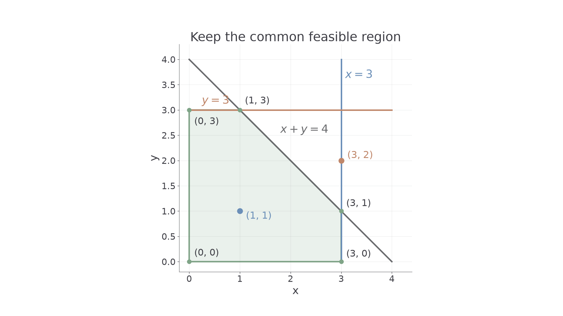
[DIAGRAM: asset_name: The common region of five bounds; asset_slug: lp_feasible_pentagon; caption: All five restrictions contribute to checking feasibility; description: Axes x and y show the region x at least zero, y at least zero, x at most 3, y at most 3, x plus y at most 4. The feasible pentagon is pale sage with vertices (0,0), (3,0), (3,1), (1,3), (0,3) labelled. Boundaries x equals 3, y equals 3 and x plus y equals 4 are labelled clear of their intersections. A blue point (1,1) is feasible and a clay point (3,2) lies outside the sloping boundary.]
All five restrictions contribute to checking feasibility

Worked example 1: intersecting half-planes

Question. Identify the feasible region for

x,y\ge0,\qquad x\le3,\qquad y\le3,\qquad x+y\le4

Plan. Start with the first-quadrant square and retain the side of $x+y=4$ containing the origin.

\begin{aligned} x=3,\quad x+y=4&\ \Longrightarrow\ y=1&&\text{right sloping intersection}\\ y=3,\quad x+y=4&\ \Longrightarrow\ x=1&&\text{upper sloping intersection} \end{aligned}

Why this step? The common region must satisfy both individual caps and the total cap, not whichever one looks most restrictive in isolation.

Answer. The feasible pentagon has vertices $(0,0),(3,0),(3,1),(1,3),(0,3)$ , including its edges.

Check. $(1,1)$ satisfies all bounds. $(3,2)$ meets the individual caps but fails $x+y\le4$ .

Change only the model by adding one lower bound.

Worked example 2: contradictory bounds

Question. Add $x+y\ge5$ to Example 1. Identify the resulting feasible region.

Plan. Compare the new bound with the existing total upper bound.

5\le x+y\le4

Why this step? No real number can satisfy both bounds, regardless of the individual caps.

Answer. The feasible region is empty, so the LP is infeasible.

Check. Even the original region's largest possible total $x+y=4$ fails the new lower bound.

Check every inequality before evaluating the objective. A large profit at an infeasible point is not a candidate solution.

Watch out

Wrong: omit the axes or a transformed non-negativity constraint from the diagram. Right: show the common feasible region with all its boundaries.

Make the added bound just attainable.

Objective lines and vertex checking

For a non-empty bounded polygon, a linear objective has an optimum at at least one vertex. Other optimal points may exist too.

Objective lines

For $P=ax+by$ , with $b\ne0$ , a fixed objective value gives

y=-\frac abx+\frac Pb

The objective lines are parallel. Move them in the direction of increasing $P$ for maximisation, or evaluate the objective at every feasible vertex.

Not in the formula booklet: learn it.

A graphical solution needs both a feasible optimal point and its objective value. Listing a number without identifying its point leaves the decision unfinished.

Worked example 3: maximising one profit function

Question. For the pentagon of Example 1, maximise $P=3x+2y$ .

Plan. Evaluate all five vertices, or slide lines of gradient $-3/2$ to the last feasible contact.

Vertex	$P=3x+2y$
$(0,0)$	$0$
$(3,0)$	$9$
$(3,1)$	$11$
$(1,3)$	$9$
$(0,3)$	$6$

P(3,1)=3(3)+2(1)=11

Why this step? A sloping resource boundary can make a mixed plan beat either axis intercept.

Answer. The maximum is $11$ , at $(x,y)=(3,1)$ .

Check. This point satisfies $x+y=4$ and both individual caps; no listed feasible vertex gives a larger value.

Change only the objective coefficients.

Worked example 4: the same region, a different objective

Question. Keep the same feasible pentagon, but maximise $P=2x+3y$ .

Plan. Retain the vertices and recalculate their objective values.

Vertex	$P=2x+3y$
$(0,0)$	$0$
$(3,0)$	$6$
$(3,1)$	$9$
$(1,3)$	$11$
$(0,3)$	$9$

P(1,3)=2(1)+3(3)=11

Why this step? A change to profit affects which feasible point is best, even when no resource limit changes.

Answer. The maximum is $11$ , now at $(1,3)$ .

Check. Exchanging the two coefficients exchanges the preferred coordinate in this symmetric region.

Use enumeration when a sketch's objective-line position is difficult to distinguish; use the sketch to ensure your list contains every vertex.

Watch out

Wrong: test only the intercepts on the axes. Right: include intersections of constraint boundaries inside the first quadrant.

Change the objective again.

Changed models and special outcomes

Changing a constraint changes the feasible set; changing the objective changes how points in that set are compared.

Relaxing a constraint cannot lower an attained maximum when the objective is unchanged, because the old feasible plans remain available. Tightening it cannot raise that maximum. A change may have no effect.

Worked example 5: relaxing a cap

Question. Maximise $P=4x+y$ under $x,y\ge0$ , $x+y\le4$ , $y\le3$ . Compare the cases $x\le3$ and $x\le4$ .

Plan. Identify the new right-hand vertex and compare objective values.

\begin{aligned} x\le3:&\quad P(3,1)=13&&\text{original optimum}\\ x\le4:&\quad (4,0)\text{ is now feasible}&&\text{relaxed cap}\\ P(4,0)&=16&&\text{new objective value} \end{aligned}

For the relaxed region, the other vertices $(0,0),(1,3),(0,3)$ give $0,7,3$ .

Why this step? Relaxing a binding cap can expose a better point. Reusing the old optimum without checking the new boundary would miss it.

Answer. The maximum rises from $13$ at $(3,1)$ to $16$ at $(4,0)$ .

Check. The old point remains feasible, so the new maximum cannot be less than $13$ .

Retain the relaxed region and change only the objective.

Worked example 6: more than one optimal point

Question. For $x,y\ge0$ , $x\le4$ , $y\le3$ , $x+y\le4$ , maximise $P=x+y$ .

Plan. Compare the objective with the total constraint and identify all feasible points attaining its bound.

\begin{aligned} P&=x+y\le4&&\text{objective has a direct upper bound}\\ x+y&=4,\quad 0\le y\le3&&\text{feasible equality points}\\ (x,y)&=(4-y,y)&&\text{whole optimal segment} \end{aligned}

Why this step? The objective line is parallel to, and at the optimum coincides with, a feasible boundary edge.

Answer. The maximum is $4$ , attained at every point of the segment from $(4,0)$ to $(1,3)$ .

Check. Both endpoints give $4$ , as does their midpoint $(2.5,1.5)$ .

A redundant constraint adds no restriction to the feasible set: adding $x\le5$ to the region above does nothing. Multiple optimal points concern equal objective values at different feasible points, rather than a redundant constraint.

An unbounded objective can improve without limit. With only $x,y\ge0$ , maximising $x+y$ is unbounded. An unbounded region need not imply that outcome: on the same region, maximising $-x-y$ has maximum $0$ at the origin.

Watch out

Wrong: conclude that every unbounded region has no optimum, or that an unchanged optimum makes every added constraint redundant. Check the feasible set and objective separately.

Tighten the cap and retain the first objective.

Integer solutions and the limits of rounding

An integer solution must be a feasible lattice point, with integer coordinates. Solve the continuous relaxation for guidance, then check the actual integer candidates.

Continuous relaxation

The continuous relaxation drops an LP's integer requirement but retains its other constraints. For a maximisation problem, its optimal value is an upper bound on the integer optimum, because it permits at least all the integer plans.

Rounding can violate a constraint, and rounding down can discard a better feasible plan. The opening puzzle is an example.

Continue this lesson.

You’re previewing NovaLearn without an account. Create a free account to read the rest.

Create free account

Last Accessed

Core Pure

Mechanics (Major and Minor)

Statistics (Major and Minor)

Modelling with Algorithms

Numerical Methods

Extra Pure

Further Pure with Technology

AL7–AL11 - Graphical solution of linear programs

Drawing the feasible region

Objective lines and vertex checking

Changed models and special outcomes

Integer solutions and the limits of rounding

Continue this lesson.

Learn faster with Nova