Ne3, Ne4, NU7 - Order of convergence and failure | OCR A-Level Further Mathematics B (MEI)

Interpret error and difference columns, distinguish sequence convergence from step-length order, and recognise when an iteration is slow or fails. You will compare computational costs and investigate why Newton-Raphson is generally, rather than invariably, second order.

Compare the next error with the current error

Newton-Raphson is famous for rapid convergence. Can changing $x^2-2=0$ to the equivalent equation $(x^2-2)^2=0$ make its approach much slower?

The roots are unchanged, but the curve is flatter at them. We will inspect actual output, after defining precisely what “faster” means.

You already know

The signed error is $e_n=x_n-\alpha$ , where $\alpha$ is the exact target. Use $|e_n|$ when comparing error magnitudes. A change $x_{n+1}-x_n$ is not the same quantity as the error.

A convergent sequence approaches a finite limit; a divergent sequence does not. Divergence includes an unbounded sequence and an endless cycle between different values.

Order of an iterative sequence

Near the limit, order $p$ is described by

|e_{n+1}|\approx C|e_n|^p

with a non-zero limiting constant $C>0$ . In the usual geometrically convergent first-order cases here, $p=1$ and $0<C<1$ . For second order, $p=2$ . Test candidate powers by examining $|e_{n+1}|/|e_n|^p$ in sufficiently late output.

Not in the formula booklet: learn it.

If the limit is unknown, a spreadsheet often uses $\Delta_n=x_{n+1}-x_n$ . A signed ratio $\Delta_{n+1}/\Delta_n$ tending to a non-zero magnitude below one supports first order; a non-zero finite limit of $\Delta_{n+1}/\Delta_n^2$ supports second order. This is evidence from late differences, not a demand that early ratios be exactly constant.

An order need not be an integer. For example, ordinary difference ratios decreasing towards zero while squared-difference ratios grow in magnitude can suggest convergence faster than first order but slower than second order. Report what sufficiently late output supports; do not force every sequence into one of two labels.

Worked example 1: first-order errors

Question. A sequence approaching $2$ has values $2.2,2.1,2.05,2.025$ . Identify the apparent order and predict the next value if its error pattern continues.

Plan. Subtract the known limit, then compare successive errors.

\begin{aligned} e_0,e_1,e_2,e_3&=0.2,\ 0.1,\ 0.05,\ 0.025 && \text{signed errors}\\ e_1/e_0=e_2/e_1=e_3/e_2&=0.5 && \text{constant first-power ratio}\\ e_4&=0.5(0.025)=0.0125 && \text{continue the pattern}\\ x_4&=2.0125 && \text{restore the limit} \end{aligned}

Why this step? The shrinking errors, not the ratios $x_{n+1}/x_n$ , determine convergence order.

Answer. First order, with predicted next value $2.0125$ .

Check. The first changes are $-0.1,-0.05,-0.025$ ; their consecutive ratios are also $0.5$ .

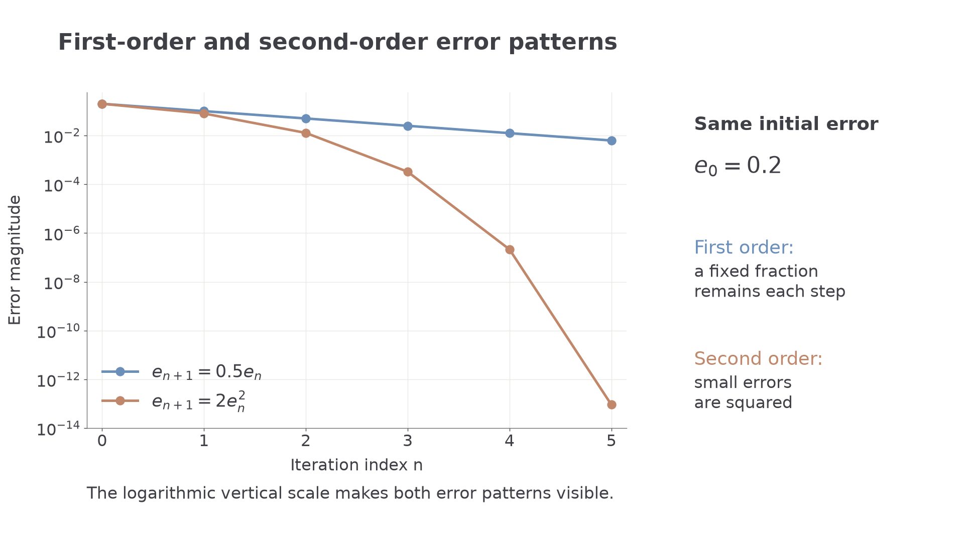
Change only the error-update pattern: retain the same limit and initial value, but let each new error be twice the square of its predecessor.

Worked example 2: second-order errors

Question. The values are now $2.2,2.08,2.0128,2.00032768$ . Identify the order and predict the next value under the stated pattern.

Plan. Compare the next error with the square of the previous error.

\begin{aligned} e_0,e_1,e_2,e_3&=0.2,\ 0.08,\ 0.0128,\ 0.00032768 && \text{same exact limit}\\ \frac{0.08}{0.2^2} =\frac{0.0128}{0.08^2} =\frac{0.00032768}{0.0128^2}&=2 && \text{quadratic ratios}\\ e_4&=2(0.00032768)^2=0.0000002147483648 && \text{next error}\\ x_4&=2.0000002147483648 && \text{next approximation} \end{aligned}

Why this step? Ordinary error ratios now decrease towards zero; treating zero as a first-order constant would miss the higher order.

Answer. Second order, with the predicted value above.

Check. Continuing this pattern, the later squared-difference ratios are approximately $-2.10509,-2.00262,-2.00000$ , approaching a non-zero constant as expected.

Squaring an already small error can remove several decimal places of error in one step. It does not mean “perform twice as many iterations”.

[DIAGRAM: asset_name: First-order and second-order error patterns; asset_slug: sequence_error_orders; caption: Squaring small errors changes how rapidly their magnitudes fall; description: A logarithmic vertical axis shows error magnitude against iteration index for the two worked sequences starting with error 0.2. The first-order sequence halves its error each time. The second-order sequence uses twice the squared previous error and bends sharply downwards. Both axes and the two rules are labelled.]
Squaring small errors changes how rapidly their magnitudes fall

Watch out

Wrong: call a sequence second order because its errors get smaller, or because two digits agree. Right: test the appropriate error or difference ratios and inspect whether they settle to a non-zero constant.

Here the exact limit is unavailable, so use the supplied difference column.

Order of a method is measured against step length

For a method controlled by a step length $h$ , the question is different: how does its error scale as $h$ decreases?

Order with respect to step length

A method is order $k$ if, in the relevant small-step regime,

|E(h)|\approx K h^k,\qquad K>0

Halving $h$ should then multiply error magnitude by approximately $2^{-k}$ . This is not the same definition as $|e_{n+1}|\approx C|e_n|^p$ .

Not in the formula booklet: learn it.

A sequence of approximations obtained by halving $h$ can therefore have first-order sequence convergence even when the underlying method is fourth order. The two uses of “order” compare different quantities.

Worked example 3: a second-order method

Question. A method approximates a true value $2$ . Its errors satisfy $E(h)=3h^2$ , with $h=0.2,0.1,0.05$ . Find its method order and the sequence order of these approximations as $h$ is repeatedly halved.

Plan. Calculate the errors, then distinguish their dependence on $h$ from their dependence on the preceding error.

\begin{aligned} E(h)&=0.12,\ 0.03,\ 0.0075 && \text{evaluate }3h^2\\ A(h)&=2.12,\ 2.03,\ 2.0075 && \text{approximate values}\\ E(h/2)/E(h)&=\frac14 && \text{error multiplier per halving} \end{aligned}

Why this step? The exponent of $h$ is two, but one sequence error is one quarter of its predecessor.

Answer. Second-order method; first-order convergence of the halving-generated sequence, with factor $1/4$ .

Check. $2^{-2}=1/4$ , agreeing with the method-order prediction.

Change only the power of $h$ from two to four; retain the constant, true value and step lengths.

Worked example 4: a fourth-order method

Question. Repeat the interpretation when $E(h)=3h^4$ .

Plan. Recalculate the errors and their ratio for halved steps.

\begin{aligned} E(h)&=0.0048,\ 0.0003,\ 0.00001875 && \text{evaluate }3h^4\\ A(h)&=2.0048,\ 2.0003,\ 2.00001875 && \text{same true value}\\ E(h/2)/E(h)&=\frac1{16} && \text{constant sequence factor} \end{aligned}

Why this step? A constant non-zero ratio of consecutive errors is first-order sequence convergence, even when that constant is very small.

Answer. Fourth-order method; still first-order sequence convergence, now with factor $1/16$ .

Check. $2^{-4}=1/16$ . Calling the sequence itself fourth order would compare each new error with the fourth power of the old one, which these data do not support.

Later differentiation and integration lessons apply this distinction to concrete numerical methods. Here the supplied error models make the two meanings visible without a formal expansion.

Watch out

Wrong: transfer an order label from a method directly to any sequence generated by changing its step length. Right: say which variable is being compared with the error.

Read a new approximation table.

A local gradient explains the iteration pattern

For a smooth fixed-point map near $\alpha$ , its gradient gives a useful local guide. The start must be close enough and the iterates must remain in the relevant domain.

Gradient at the fixed point	Typical nearby behaviour
$0<g'(\alpha)<1$	Approaches from one side; first order
$-1<g'(\alpha)<0$	Alternates across the fixed point; first order
$	g'(\alpha)
$g'(\alpha)=0$	Higher-order convergence may occur; inspect the output
$	g'(\alpha)

A factor close in magnitude to one gives slow progress. A negative gradient of magnitude $0.98$ , for instance, suggests alternating errors that shrink only slightly each step.

These local gradient guides and the general first-order behaviour of fixed point iteration are not printed in the formula booklet. They do not guarantee convergence from a distant starting point. Starting exactly at a fixed point leaves it unchanged even if nearby points are repelled.

Continue this lesson.

You’re previewing NovaLearn without an account. Create a free account to read the rest.

Create free account

Last Accessed

Core Pure

Mechanics (Major and Minor)

Statistics (Major and Minor)

Modelling with Algorithms

Numerical Methods

Extra Pure

Further Pure with Technology

Ne3, Ne4, NU7 - Order of convergence and failure

Compare the next error with the current error

Order of a method is measured against step length

A local gradient explains the iteration pattern

Continue this lesson.

Learn faster with Nova