SH6 - Hypothesis tests for a mean
SH6 tests a single population mean using a Normal or reference distribution. You will choose the distribution from the sampling conditions, distinguish one- and two-sided alternatives, use the right critical-value convention, and state what the evidence suggests in context.
Choose the question and model before calculating
Can the same sample give a significant one-sided result but a non-significant two-sided result? Yes. At the level, a positive standardised statistic exceeds the one-sided Normal cutoff , but not the two-sided cutoff .
This is not permission to choose the alternative after seeing the data. The alternative must reflect the question you set out to investigate.
You already know
The sampling distribution concerns the sample mean. Standard error is , estimated by when necessary. Small Normal samples with unknown variance use , as in confidence intervals.
Define as the population mean of the measurement in context. Use , and choose , , or according to the claim. A hypothesis about would concern a number already observed.
| Sampling conditions | Reference distribution |
|---|---|
| Normal population, known population variance | Normal, exact under the model, at any sample size |
| Large independent sample, finite variance | Normal approximation, using if the population variance is unknown |
| Small independent sample, Normal population, unknown variance | with degrees of freedom |
For a small sample with no justified Normal model, a test is not automatically appropriate. A signed rank test addresses a median and needs symmetry; it cannot be substituted without checking what parameter the question asks about.
Watch out
Wrong: “The population is Normal, so use a Normal test even though its variance is unknown and the sample is small.”
Right: use in that case. Population Normality and knowledge of the population variance are separate conditions.
Choose a reference distribution for a specified design.
Standardise a mean using the null hypothesis
The null model tells you how surprising the observed mean would be if the proposed population mean were correct. Use , not a fitted alternative mean, in the numerator.
Normal test statistic for a mean
For a Normal sampling distribution with known standard error, under ,
Calculate the observed statistic using . For an exact small-sample Normal test, the underlying population must be Normal and known.
In the formula booklet.
The booklet's percentage-point table gives total two-tail percentages. For a one-sided upper test, use , from its total-tail column. For a two-sided test, use , from its column. Reverse the sign for a lower-sided test.
Worked example 1: a one-sided Normal test
Question. A Normal population of instrument readings has known standard deviation . A random independent sample of readings has mean . Test at the level whether the population mean exceeds .
Plan. Standardise using the known spread and compare with the upper one-sided cutoff.
Why this step? A larger-mean alternative asks whether the observed mean is unusually far above the null value, so only the upper tail counts.
Answer. Reject . There is sufficient evidence at the level to suggest that the population mean reading exceeds .
Check. The one-sided tail probability is approximately , agreeing with the critical-value decision.
Change only the alternative: suppose the investigation asks whether the mean differs from .
Worked example 2: the same statistic in a two-sided test
Question. For the same sample, test against at the level.
Plan. Retain the statistic , but split the significance level between both tails.
Why this step? A two-sided test must allow for a discrepancy in either direction, so its upper cutoff is further from zero.
Answer. Do not reject . There is insufficient evidence at the level to suggest that the population mean differs from .
Check. The two-sided -value is about .
[DIAGRAM: asset_name: One statistic against one-sided and two-sided cutoffs; asset_slug: h645_b107_tails; caption: A statistic of one point eight is in the one-sided five percent rejection region but outside the two-sided five percent regions; description: Two standard Normal curves show upper five percent shading beyond one point six four five in the first panel, and two point five percent shading beyond plus and minus one point nine six in the second. A vertical clay line marks statistic one point eight in both, with its position relative to the cutoffs explicitly labelled.]
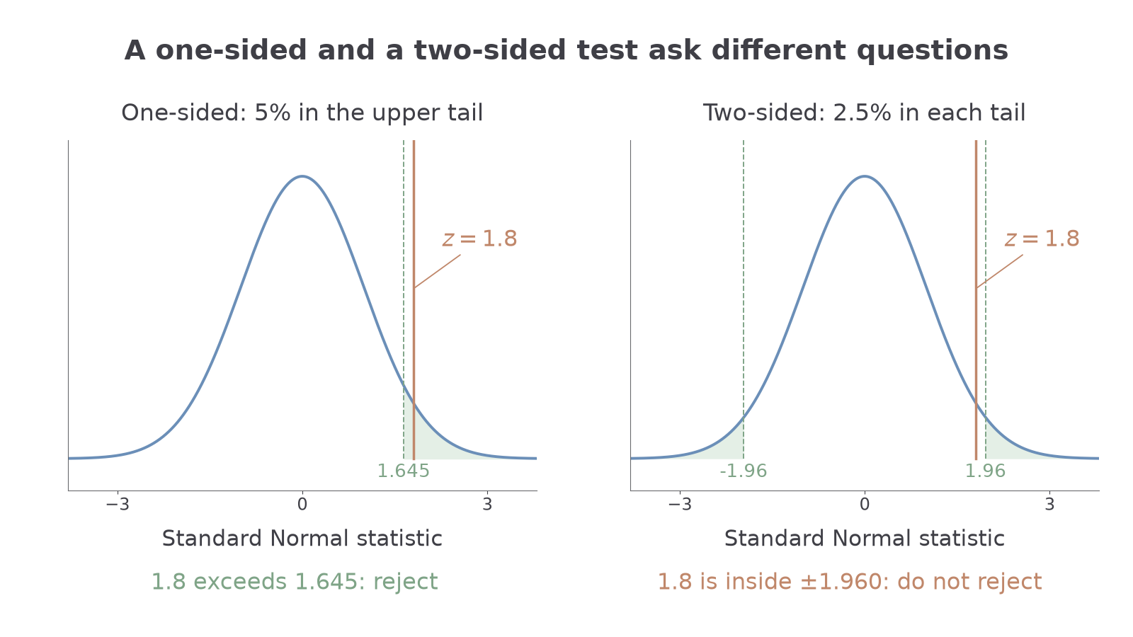
For a lower-sided claim use the lower tail: at the level reject for . A positive statistic cannot support a lower-sided alternative just because its absolute value is large.
Exam tip
Show the hypotheses, population parameter definition, statistic, reference distribution, correct tail cutoff, comparison and non-assertive conclusion. “Accept ” must not become a claim that the proposed mean has been proved.
Keep a two-sided investigation, but use a new observed mean.
Watch out
Wrong: reject the two-sided test because . That cutoff allocates to just the upper tail. Correct: use for the two-sided test; , so do not reject.
Match the next alternative to its tail cutoff before comparing the statistic.
A large sample allows an estimated Normal standard error
When the population variance is unknown but the independent sample is sufficiently large, use the CLT for the mean and estimate its standard error by . This is an approximate Normal procedure, rather than the exact known-variance calculation.
Continue this lesson.
You’re previewing NovaLearn without an account. Create a free account to read the rest.
Create free account