SR30, SR31 - Checking a Normal model
SR30 distinguishes a Normal model for individual observations from a Normal approximation for a sampling distribution. SR31 uses supplied Normal probability plots and Kolmogorov-Smirnov output to judge a proposed fit. You will interpret evidence cautiously, without constructing the plots or calculating the test statistic.
What quantity is supposed to be Normal?
A hospital's waiting times are strongly right-skewed, but a simulation shows a roughly bell-shaped distribution of averages from repeated large independent samples. Has the simulation shown that individual waiting times are Normal?
No. It has changed the random quantity being studied. A single waiting time and a mean of many waiting times have different distributions. Taking more observations does not turn the original population into a Normal population.
You already know
A Normal model is symmetric, bell-shaped and unbounded. Independent observations from a Normal population have an exactly Normal sample mean, for any positive sample size. Exact Normality of those observations is an assumption, not a consequence of averaging.
For an individual measurement, consider the context and observed shape. A fairly symmetric, single cluster with no marked outliers may support a Normal model. Strong skewness, distinct clusters or a few very large outliers cast doubt on it. A non-negative quantity is not automatically unsuitable: the practical issue is whether a proposed Normal model gives appreciable probability to impossible negative values.
Normal model and Normal approximation
A Normal population model describes individual observations themselves as Normally distributed.
A Normal approximation uses a Normal distribution as a convenient approximation to another distribution. In the context of the Central Limit Theorem, sufficiently large averages of independent observations from the same population, with finite mean and variance, can be approximately Normal even when the original observations are not.
There is no sample size that makes every possible population shape harmless. Strong skewness may need a larger sample, and dependence can undermine the independent-observation argument. Detailed sample-mean calculations belong to the later inference methods; the decision here is which random quantity and assumptions justify considering a Normal model.
Key idea
“Individual observations are Normal” and “a large-sample average is approximately Normal” are different claims. Evidence for the second does not establish the first.
The hospital example is a useful surprise: averaging can produce a nearly symmetric shape while every individual waiting-time distribution remains skewed.
Judge whether the supplied points follow a straight line
A Normal probability plot compares ordered sample values with expected Normal values. Different software may reverse the axes or use different conventions. Read the labels; the essential comparison is still with a straight line.
The closer the points lie to a straight line, the more plausible a Normal fit. Small random departures are expected. A sustained curve or a conspicuous departure at an end raises concern. You only need to judge the supplied plot by eye, not construct it or calculate its coordinates.
[DIAGRAM: asset_name: Two supplied Normal probability plots; asset_slug: h645_b101_plots_ab; caption: Plot A is close to a straight line; Plot B has a clear systematic curve; description: Two Normal probability plots have sample values on the horizontal axes and expected standard Normal values on the vertical axes. Plot A has points close to a rising straight reference line. Plot B has a sustained curved pattern that departs substantially from a straight reference line. The plots are labelled A and B without claiming that a straight appearance proves Normality.]
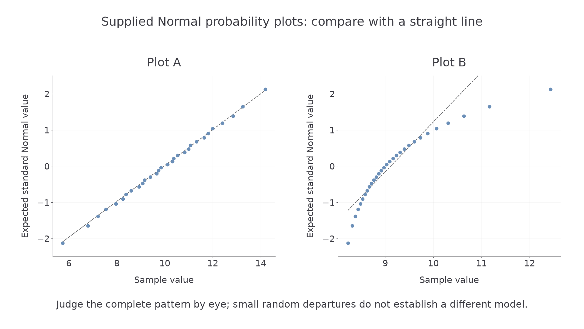
Worked example 1: a plausible fit
Question. An investigator produces Plot A from a random sample of a measurement. Comment on whether a Normal model might be appropriate.
Plan. Compare the overall pattern with a straight line, then state what that evidence permits.
Step 1. The points lie close to a straight line, with small departures rather than a sustained bend.
Step 2. There is no marked isolated point or systematic curvature in this plot.
Why this step? An approximately straight pattern is the feature expected from a Normal fit. It supports considering the model, but a finite sample cannot prove a population distribution.
Answer. The plot is approximately straight, suggesting that a Normal model may be appropriate for these observations.
Check. The conclusion is about a possible population model, not a claim that the observed points must lie exactly on a line.
Change only the pattern in the supplied plot: Plot B bends systematically away from a straight line.
Worked example 2: systematic curvature
Question. An investigator instead obtains Plot B. Comment on the proposed Normal model.
Plan. Identify a sustained departure from straightness and connect it to model suitability.
Step 1. The points follow a clear curve, rather than showing small irregular departures around a straight line.
Step 2. The discrepancy affects much of the plot, so it is not just one small plotting fluctuation.
Why this step? A systematic bend is evidence against a good Normal fit. No calculation of the slope, correlation or individual plot coordinates is required.
Answer. The substantial curvature suggests that a Normal model is unlikely to be suitable for these observations.
Check. The axes show individual sample values and expected Normal values. This is not a scatter diagram of two measured variables, so a correlation test is not the relevant interpretation.
Do not infer a particular named alternative distribution from curvature alone. The task is to assess the proposed Normal fit, using the feature visible in the supplied graph.
Watch out
Wrong: “the points rise, so the data are Normal”. Right: judge proximity to a straight line. A rising curve can still show substantial disagreement with a Normal model.
Continue this lesson.
You’re previewing NovaLearn without an account. Create a free account to read the rest.
Create free account