Ne5 - Relaxation of fixed point iteration | OCR A-Level Further Mathematics B (MEI)

Use relaxation to change the behaviour of a fixed-point iteration. You will compare supplied parameters, accelerate a convergent sequence and turn a repelling fixed point into an attracting one, while checking accuracy and domains.

Blend the old value with the proposed new value

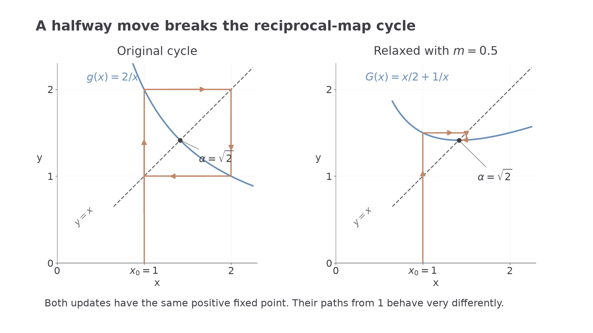
The iteration $x_{n+1}=2/x_n$ , starting at $1$ , cycles $1,2,1,2,\ldots$ . What if each step moves only halfway towards the proposed next value?

That small change breaks the cycle. More surprisingly, the resulting formula is exactly Newton-Raphson's update for the positive square root of $2$ .

You already know

A fixed point satisfies $\alpha=g(\alpha)$ . Local gradients and iteration output help judge convergence. Keep stored precision between steps; a rounded display is not a new input.

Relaxation changes the update rule while retaining its intended fixed points.

Relaxation

Replace $x_{n+1}=g(x_n)$ by

x_{n+1}=G_m(x_n)=(1-m)x_n+m g(x_n)

where $m$ is the relaxation parameter. For $m\ne0$ , the fixed-point equations are equivalent:

x=G_m(x) \quad\Longleftrightarrow\quad mx=mg(x) \quad\Longleftrightarrow\quad x=g(x)

within the original domain. At $m=1$ , the original iteration is recovered. At $m=0$ , every starting value stays unchanged, so this is not a useful root-finding iteration.

In the formula booklet.

For $0<m<1$ , the new value is a weighted average of the old value and the unrelaxed proposal. Relaxation also permits parameters outside this interval; we will meet a useful negative one later.

Worked example 1: stop a two-cycle

Question. Use $m=0.5$ to relax $g(x)=2/x$ , with $x_0=1$ . Calculate four iterates and find the positive fixed point to $4$ decimal places.

Plan. Substitute the parameter before iterating, retain precision, then certify the proposed rounded root.

\begin{aligned} G_{0.5}(x)&=0.5x+0.5\left(\frac2x\right) =\frac{x}{2}+\frac1x && \text{form the actual update}\\ x_1&=\frac12+1=1.5 && \text{start at }1\\ x_2&=\frac{1.5}{2}+\frac1{1.5} =\frac{17}{12} && \text{reuse the full value}\\ x=G_{0.5}(x)&\Longrightarrow x^2=2 && \text{identify the fixed points} \end{aligned}

$n$	Displayed $x_n$ , $8$ d.p.
$1$	$1.50000000$
$2$	$1.41666667$
$3$	$1.41421569$
$4$	$1.41421356$

Why this step? Average the old value and the proposal before making the next update; averaging two already rounded displays would create a different calculation.

Answer. The positive fixed point is $1.4142$ to $4$ decimal places.

Check. For $f(x)=x^2-2$ ,

f(1.41415)=-0.0001797775<0,\qquad f(1.41425)=0.0001030625>0

Continuity and strict increase on this positive interval put the unique root inside the rounding interval for $1.4142$ . All iterates remain positive, so division by zero is avoided.

Change only the parameter to $0.25$ , retaining the same map and seed.

Worked example 2: a smaller move is slower here

Question. Calculate four iterates with $m=0.25$ . Compare the approach with $m=0.5$ .

Plan. Rebuild the relaxed formula, then run it from the original seed.

\begin{aligned} G_{0.25}(x)&=0.75x+\frac{0.5}{x} && \text{new weights}\\ x_1&=0.75(1)+0.5=1.25 && \text{reset the seed}\\ x_2&=0.75(1.25)+\frac{0.5}{1.25} =1.3375 && \text{second step} \end{aligned}

$n$	Displayed $x_n$ , $8$ d.p.
$1$	$1.25000000$
$2$	$1.33750000$
$3$	$1.37695678$
$4$	$1.39583719$
$12$	$1.41414271$
$13$	$1.41417814$

Why this step? “More cautious” does not mean “faster”: the changed parameter makes much smaller corrections near this fixed point.

Answer. This output approaches the same positive fixed point more slowly. The $m=0.5$ trace already supports the certified $4$ -decimal-place result after four steps; the $m=0.25$ trace takes substantially longer.

Check. For any positive fixed point,

x=0.75x+\frac{0.5}{x} \Longrightarrow 0.25x^2=0.5 \Longrightarrow x^2=2

The target has not changed. The rounding certificate from example 1 still applies; repeated displayed agreement alone is not that certificate.

The graph shows how averaging changes the path, rather than merely changing the printed digits.

[DIAGRAM: asset_name: Relaxation breaks a reciprocal-map cycle; asset_slug: relaxation_breaks_cycle; caption: Halfway moves turn the reciprocal two-cycle into a convergent path; description: Two equal-scale panels show the identity line, the original map y=2/x and the relaxed map y=x/2+1/x for positive x. Vertical-horizontal moves from x0=1 cycle between 1 and 2 in the original panel but approach the common positive fixed point square root of 2 in the relaxed panel. The two update rules and seed are labelled.]
Halfway moves turn the reciprocal two-cycle into a convergent path

Watch out

Wrong: assume smaller $m$ always gives faster convergence. Right: compare the new map's behaviour, the starting value and actual output. The best of two supplied choices depends on the equation.

Try a third parameter without changing the root problem.

Compare parameters using gradients and output

An iteration can already converge and still benefit greatly from relaxation. For $g(x)=\cos x$ , using radians, the fixed point near $0.739$ has $g'(\alpha)\approx-0.673612$ . The unrelaxed path alternates, with a substantial fraction of its error left after each step.

Gradient of the relaxed map

For a differentiable map,

G_m'(\alpha)=1-m+m g'(\alpha)

A magnitude below one supports local convergence; a small magnitude usually gives faster local error reduction. A negative gradient suggests alternation and a positive one a same-side approach. The gradient test alone is inconclusive at magnitude one, and it does not guarantee success from a distant start.

Not in the formula booklet: learn it.

Use the gradient to interpret supplied parameter choices, then check the actual sequence. There is no need to derive an optimal parameter.

Worked example 3: damp an alternating approach

Question. Starting at $x_0=1$ , use $m=0.5$ for $g(x)=\cos x$ . Calculate four iterates and explain why this should improve the local rate.

Plan. Form the relaxed map, use radians throughout, and compare its gradient with the original one.

\begin{aligned} G_{0.5}(x)&=0.5x+0.5\cos x && \text{relaxed update}\\ x_1&=0.5+0.5\cos1=0.77015115\ldots && \text{first step}\\ x_2&=0.5x_1+0.5\cos x_1=0.74397830\ldots && \text{retain the first value}\\ G_{0.5}'(\alpha)&\approx0.5+0.5(-0.673612) =0.163194 && \text{smaller positive factor} \end{aligned}

$n$	Displayed $x_n$ , $8$ d.p.
$1$	$0.77015115$
$2$	$0.74397830$
$3$	$0.73987925$
$4$	$0.73921461$

Why this step? Compare the gradient of the relaxed map with the gradient of $g$ , because the relaxed map generates the new sequence.

Answer. The trace approaches the fixed point from above. The local factor about $0.163$ is much smaller in magnitude than $0.674$ , so the relaxed approach is faster near this root.

Check. Continuing with stored precision gives $x_8=0.73908523\ldots$ , $x_9=0.73908515\ldots$ and $x_{10}=0.73908514\ldots$ . These shrinking positive errors agree with the gradient prediction.

Change only $m$ to $0.6$ ; the same start makes the comparison fair.

Continue this lesson.

You’re previewing NovaLearn without an account. Create a free account to read the rest.

Create free account

Last Accessed

Core Pure

Mechanics (Major and Minor)

Statistics (Major and Minor)

Modelling with Algorithms

Numerical Methods

Extra Pure

Further Pure with Technology

Ne5 - Relaxation of fixed point iteration

Blend the old value with the proposed new value

Compare parameters using gradients and output

Continue this lesson.

Learn faster with Nova