Pc16, Pc17 - Damped oscillations | OCR A-Level Further Mathematics B (MEI)

Damping changes a repeating motion into one that settles towards equilibrium. Pc16 builds second-order models from restoring and resistive effects; Pc17 connects their auxiliary roots to under-damping, critical damping and over-damping. You will interpret graphs, distinguish actual peaks from an exponential envelope, and use observed decay to find model parameters.

Restoring effects, resistance and equilibrium

Will adding more resistance always make a displaced object return to equilibrium sooner? A little resistance removes persistent oscillation, but sufficiently strong resistance can make the return slower. The auxiliary roots will explain why.

Let $x$ measure signed displacement from a chosen reference position. A restoring contribution to acceleration has the opposite sign to $x$ , while a resistive contribution has the opposite sign to velocity. For example, acceleration $-5x-2\dot{x}$ gives

\ddot{x}+2\dot{x}+5x=0

When the object moves in the negative direction, $\dot{x}<0$ , the resistance term $-2\dot{x}$ is positive: it still opposes motion.

You already know

For $\ddot{x}+a\dot{x}+bx=0$ , solve $r^2+ar+b=0$ . Negative real parts produce decaying exponential factors. A constant right side requires a particular integral; do not omit it when choosing the equilibrium position.

A constant additional effect may move equilibrium away from the reference origin. At equilibrium both derivatives are zero, so substitute those values before deciding where the motion settles.

A damped model about equilibrium

For positive constants $k$ and $\omega_0$ , a standard free damped model is

\ddot{u}+2k\dot{u}+\omega_0^2u=0

where $u$ is displacement from equilibrium. For a model $\ddot{x}+2k\dot{x}+\omega_0^2x=F$ , with constant $F$ , equilibrium is $x_e=F/\omega_0^2$ . Setting $u=x-x_e$ gives the homogeneous equation above.

Not in the formula booklet: learn it.

The positive restoring and damping coefficients describe the stable models considered here. A negative coefficient of velocity would reinforce motion rather than oppose it.

Worked example 1: modelling acceleration from two effects

Question. Time is measured in seconds. An object's acceleration is the sum of a restoring contribution $-5x$ and a resistive contribution $-2\dot{x}$ . Form its differential equation and identify its equilibrium.

Plan. Add the stated acceleration contributions, then set velocity and acceleration to zero to find equilibrium.

\begin{aligned} \ddot{x}&=-5x-2\dot{x} && \text{add the two contributions} \\ \ddot{x}+2\dot{x}+5x&=0 && \text{collect on the left} \\ 5x_e&=0\quad\Longrightarrow\quad x_e=0 && \text{zero derivatives at equilibrium} \end{aligned}

Why this step? Displacement and velocity affect acceleration separately; the velocity term must not be absorbed into the displacement coefficient.

Answer. $\ddot{x}+2\dot{x}+5x=0$ , with equilibrium $x=0$ .

Check. For $x=1$ , $\dot{x}=-1$ , the contributions are $-5$ and $+2$ , so acceleration is $-3$ , agreeing with the equation.

Worked example 2 changes only the constant contribution to acceleration, adding $10$ . The equilibrium moves, while the equation for deviations from it stays the same.

Worked example 2: a shifted equilibrium

Question. The acceleration law becomes $\ddot{x}=-5x-2\dot{x}+10$ . Form the model, find equilibrium and write an equation for displacement $u$ from equilibrium.

Plan. Find the stationary value of $x$ , then substitute $x=u+x_e$ .

\begin{aligned} \ddot{x}+2\dot{x}+5x&=10 && \text{model equation} \\ 5x_e&=10\quad\Longrightarrow\quad x_e=2 && \text{zero derivatives} \\ x&=u+2,\quad \dot{x}=\dot{u},\quad\ddot{x}=\ddot{u} && \text{constant shift} \\ \ddot{u}+2\dot{u}+5(u+2)&=10 && \text{substitute} \\ \ddot{u}+2\dot{u}+5u&=0 && \text{constant terms cancel} \end{aligned}

Why this step? Damping concerns distance from the actual equilibrium, which need not be the position labelled zero.

Answer. The equilibrium is $x=2$ , and $u=x-2$ satisfies $\ddot{u}+2\dot{u}+5u=0$ .

Check. The constant solution $x=2$ gives $0+0+10=10$ in the original equation.

The sign of resistance is most easily checked using a negative velocity.

Watch out

Wrong: resistance is always negative. Right: the contribution is $-2k\dot{x}$ . Its sign changes when velocity changes sign, so it always opposes motion.

Build the next model before shifting its equilibrium.

Three kinds of damping

The auxiliary roots decide whether a stable damped motion oscillates repeatedly or returns without an oscillatory factor.

For $\ddot{u}+2k\dot{u}+\omega_0^2u=0$ , the roots are

r=-k\pm\sqrt{k^2-\omega_0^2}

Their real parts are negative because $k>0$ and $\omega_0>0$ . The comparison between $k$ and $\omega_0$ determines which solution family is needed.

Damping classification

For $k>0$ , $\omega_0>0$ :

\begin{array}{c|c|c} \text{Condition}&\text{Auxiliary roots}&\text{Damping}\\ \hline k<\omega_0&-k\pm \nu i,\quad \nu=\sqrt{\omega_0^2-k^2}&\text{under-damping}\\ k=\omega_0&-k\text{ repeated}&\text{critical damping}\\ k>\omega_0&\text{two distinct negative real roots}&\text{over-damping} \end{array}

The corresponding solution forms are

\begin{aligned} u&=e^{-kt}(p\cos\nu t+q\sin\nu t) && \text{under-damped}\\ u&=(p+qt)e^{-kt} && \text{critically damped}\\ u&=pe^{r_1t}+qe^{r_2t} && \text{over-damped} \end{aligned}

Not in the formula booklet: learn it.

Under-damped non-zero motion crosses equilibrium repeatedly with decreasing peaks. The other two forms have no oscillatory factor. Depending on the initial velocity, they can cross equilibrium once; “non-oscillatory” does not mean every possible solution stays on its initial side.

[DIAGRAM: asset_name: Three damping regimes from the same starting state; asset_slug: damping_three_regimes; caption: With the same restoring coefficient and initial data, stronger damping can produce a slower return; description: A graph compares solutions of u double dot plus 2k u dot plus 4u equals zero with u(0)=1 and velocity zero. The under-damped curve has k=1 and crosses equilibrium, the critical curve has k=2, and the over-damped curve has k=3 and a longer positive tail. A separate lower strip labels the auxiliary roots for all three cases and keeps the legend clear of the curves.]
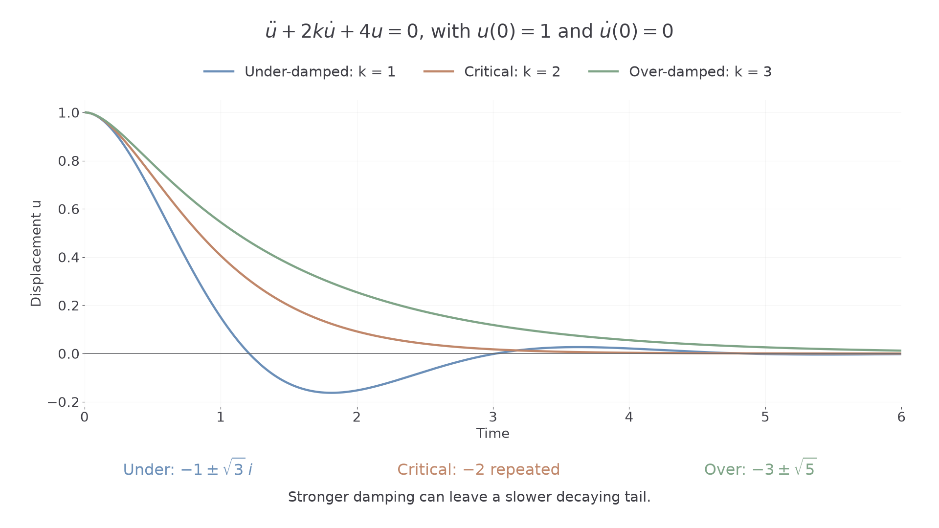
With the same restoring coefficient and initial data, stronger damping can produce a slower return

For the graph's released-from-rest comparison, critical damping returns without oscillating and avoids the long slow tail of the over-damped case. This is not a claim that every critically damped initial state beats every over-damped initial state.

Worked example 3: complex roots and oscillation

Question. Classify the damping in $\ddot{u}+2\dot{u}+4u=0$ , and describe a non-zero solution as time increases.

Plan. Solve the auxiliary quadratic and interpret its real and imaginary parts.

\begin{aligned} r^2+2r+4&=(r+1)^2+3=0 && \text{auxiliary equation} \\ r&=-1\pm\sqrt3\,i && \text{complex roots} \\ u&=e^{-t}(p\cos(\sqrt3\,t)+q\sin(\sqrt3\,t)) && \text{solution form} \end{aligned}

Why this step? The negative real part makes the size decay, while the non-zero imaginary part produces repeated oscillations.

Answer. The motion is under-damped. It crosses equilibrium repeatedly with decreasing peaks and tends to equilibrium because $e^{-t}\to0$ while the trigonometric factor is bounded.

Check. Here $k=1<\omega_0=2$ , agreeing with the classification.

Worked example 4 changes only the velocity coefficient from $2$ to $6$ . The auxiliary roots become real, and one decays much more slowly than the other.

Worked example 4: distinct real roots and a slow tail

Question. Classify the damping in $\ddot{u}+6\dot{u}+4u=0$ , and describe its long-term behaviour.

Plan. Solve the changed quadratic, check both root signs and identify the slower decaying term.

\begin{aligned} r^2+6r+4&=0 && \text{auxiliary equation} \\ r&=\frac{-6\pm\sqrt{36-16}}2=-3\pm\sqrt5 && \text{distinct real roots} \\ u&=pe^{(-3+\sqrt5)t}+qe^{(-3-\sqrt5)t} && \text{general solution} \end{aligned}

Why this step? The root $-3+\sqrt5$ is closer to zero, so its exponential decays more slowly if its coefficient is non-zero.

Answer. The motion is over-damped and non-oscillatory. Both exponentials tend to zero, so $u\to0$ . Usually the slower term governs the late return; if $p=0$ , that term is absent.

Check. Since $\sqrt5<3$ , both roots are negative. Also $k=3>\omega_0=2$ .

Between those cases, $\ddot{u}+4\dot{u}+4u=0$ has $(r+2)^2=0$ , the critical boundary. More damping has changed the root structure, not merely shrunk an otherwise unchanged sine curve.

Watch out

Wrong: “Over-damped means complex auxiliary roots.” Right: complex roots give under-damping; distinct real roots give over-damping; an equal real pair gives critical damping.

The next equation is exactly at the boundary, so its general solution needs the repeated-root factor.

Actual peaks and the exponential envelope

An under-damped solution lies inside a shrinking exponential envelope, but its local maxima generally do not touch that envelope.

Write $u=e^{-kt}(p\cos\nu t+q\sin\nu t)$ as $u=Re^{-kt}\cos(\nu t-\phi)$ , where $R=\sqrt{p^2+q^2}$ . Then $|u|\le Re^{-kt}$ . At a peak, however, the derivative of the exponential contributes as well as the derivative of the cosine. Ignoring it gives the wrong peak time.

Damped amplitude and envelope

The envelope is the pair of bounding curves $u=\pm Re^{-kt}$ . The amplitude of the damped motion refers to a local maximum distance from equilibrium; successive peaks decrease. The envelope is a bound, not usually the actual peak height at that time.

Continue this lesson.

You’re previewing NovaLearn without an account. Create a free account to read the rest.

Create free account

Last Accessed

Core Pure

Mechanics (Major and Minor)

Statistics (Major and Minor)

Modelling with Algorithms

Numerical Methods

Extra Pure

Further Pure with Technology

Pc16, Pc17 - Damped oscillations

Restoring effects, resistance and equilibrium

Three kinds of damping

Actual peaks and the exponential envelope

Continue this lesson.

Learn faster with Nova