SR24–SR26 - Cumulative distribution functions | OCR A-Level Further Mathematics B (MEI)

SR24 accumulates density into a cumulative distribution function and sketches its full shape. SR25 recovers density by differentiation. SR26 uses cumulative probabilities to find intervals, medians and percentiles, including selecting the correct branch of a piecewise function.

A cdf remembers all the probability to the left

A continuous variable has cdf $F(x)=x^2/4$ for $0\le x\le2$ . To find $P(0.5<X<1.5)$ , should you integrate this expression or subtract two of its values?

The cdf has already accumulated probability. Its height gives an area under the density, so integrating the cdf would accumulate a different quantity. First see how a cdf is built.

You already know

A pdf $f$ gives interval probabilities by integration. The area over its whole support is one. A continuous model gives $P(X=c)=0$ , so strict and inclusive endpoints give the same probability.

The lower-case $f$ and upper-case $F$ have different jobs. The cdf is dimensionless probability, whereas the pdf is density.

Cumulative distribution function

For a continuous random variable,

F(x)=P(X\le x)=\int_{-\infty}^{x}f(t)\,dt

Here $t$ is a dummy integration variable. For support $[a,b]$ , the calculation is $0$ below $a$ , $\int_a^x f(t)\,dt$ inside, and $1$ above $b$ ; the integrals used here all have finite limits.

In the formula booklet.

A continuous variable's cdf is continuous, non-decreasing, lies between zero and one, and approaches zero and one at the two ends of the real line. Flat sections mean zero density. A corner is allowed; a jump would give positive point probability and does not describe the purely continuous models here.

Worked example 1: accumulating a piecewise density

Question. A continuous variable has pdf

f(x)= \begin{cases} 1/2,&0\le x<1\\ 2-x,&1\le x\le2\\ 0,&\text{otherwise} \end{cases}

Find its cdf and describe its sketch.

Plan. Accumulate from zero, retaining the probability already collected before $x=1$ .

For $0\le x<1$ ,

F(x)=\int_0^x\frac12\,dt=\frac x2

For $1\le x\le2$ ,

\begin{aligned} F(x)&=\frac12+\int_1^x(2-t)\,dt&&\text{include the first interval}\\ &=\frac12+\left[2t-\frac{t^2}{2}\right]_1^x&&\text{integrate the second branch}\\ &=2x-\frac{x^2}{2}-1&&\text{simplify} \end{aligned}

Why this step? Beginning the second branch at zero would forget the probability $1/2$ already lying below $1$ .

Answer.

F(x)= \begin{cases} 0,&x<0\\ x/2,&0\le x<1\\ 2x-x^2/2-1,&1\le x\le2\\ 1,&x>2 \end{cases}

The sketch is flat at zero, linear up to $(1,1/2)$ , then rises with decreasing gradient to $(2,1)$ , and stays flat.

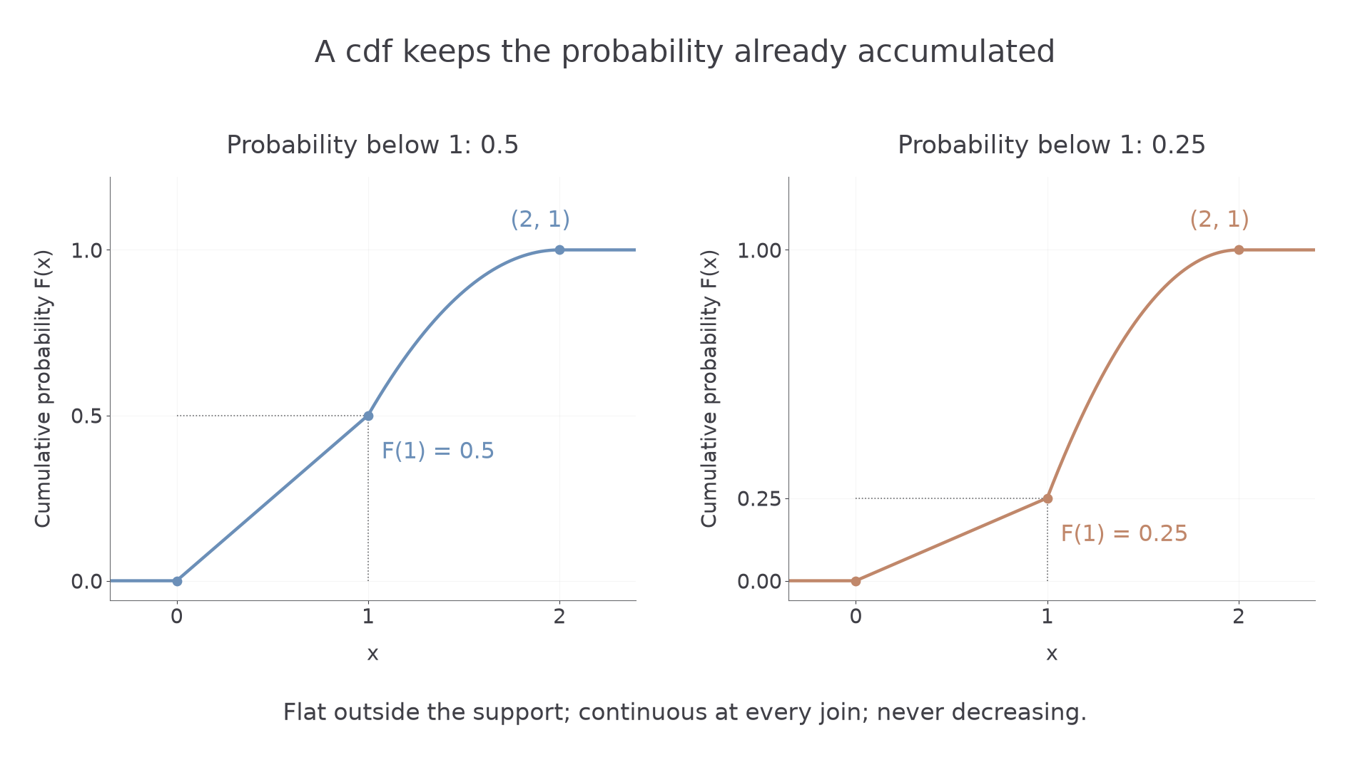
Check. Both interior branches give $1/2$ at $1$ , and the second gives $1$ at $2$ . No cumulative probability is lost at a join.

Change only how much probability lies below $1$ : it is now $1/4$ , rather than $1/2$ . The falling branch is rescaled to keep total probability one.

Worked example 2: a different branch weight

Question. Find the cdf when the pdf is $1/4$ on $0\le x<1$ , $\frac32(2-x)$ on $1\le x\le2$ , and zero otherwise.

Plan. Carry probability $1/4$ into the second branch.

\begin{aligned} F(x)&=\frac x4&&0\le x<1\\ F(x)&=\frac14+\int_1^x\frac32(2-t)\,dt&&1\le x\le2\\ &=\frac14+\frac32\left(2x-\frac{x^2}{2}-\frac32\right)&&\text{evaluate}\\ &=3x-\frac{3x^2}{4}-2&&\text{simplify} \end{aligned}

Why this step? The second formula must start at $1/4$ and rise by the remaining $3/4$ , not restart at zero.

Answer.

F(x)= \begin{cases} 0,&x<0\\ x/4,&0\le x<1\\ 3x-3x^2/4-2,&1\le x\le2\\ 1,&x>2 \end{cases}

The sketch passes through $(0,0)$ , $(1,1/4)$ and $(2,1)$ , with constant exterior branches.

Check. $F(1)=3-3/4-2=1/4$ and $F(2)=6-3-2=1$ , so both joins are continuous.

The cdf's final plateau is one, but its area is not required to be one. In fact its right-hand plateau continues indefinitely. The area-one condition belongs to the pdf.

[DIAGRAM: asset_name: Accumulating piecewise density without resetting; asset_slug: h645_b099_piecewise_cdf; caption: The cdf keeps its accumulated probability when the pdf changes rule; description: Two panels plot the complete cdfs from the worked examples, including flat zero and one branches. The first passes through one, one half and the second through one, one quarter. Each panel marks the join at x equals one and the endpoint at two, one, with labels placed outside the curves.]
The cdf keeps its accumulated probability when the pdf changes rule

Watch out

Wrong: use only $\int_1^x f(t)\,dt$ after the breakpoint. Right: add $F(1)$ . The second formula must join the first continuously.

Move the probability weight below $1$ to $3/4$ .

Differentiate the cdf and check the whole support

A cdf's gradient measures how quickly probability is accumulating. A steep section means a large density; a flat section means no probability is being added.

Density from a cdf

Where the cdf is differentiable,

f(x)=F'(x)

Differentiate each branch over its own interval. On a constant exterior branch, the density is zero. A density value at an isolated corner or endpoint can be chosen without changing any probability.

This follows from the supplied cdf integral; the derivative form is not printed separately.

Not in the formula booklet: learn it.

To establish that a proposed continuous cdf is valid, check its joins and endpoint values as well as its gradient. Showing that a few sampled values rise is not a proof that the entire function is non-decreasing.

Worked example 3: recovering a linear density

Question. A function is defined by $F(x)=0$ for $x<0$ , $F(x)=x^2/4$ for $0\le x\le2$ , and $F(x)=1$ for $x>2$ . Show that it is a valid continuous cdf and find a corresponding pdf.

Plan. Check continuous joins and non-negative derivative, then differentiate the interior branch.

\begin{aligned} F(0)&=0,\qquad F(2)=1&&\text{joins and limiting values}\\ F'(x)&=\frac x2\ge0\quad(0<x<2)&&\text{non-decreasing on the support}\\ f(x)&=\frac x2\quad(0<x<2)&&\text{density is the gradient} \end{aligned}

Why this step? Correct endpoint values alone do not rule out a dip or an overshoot between them. The derivative establishes monotonicity throughout the interval.

Answer. The function is continuous, non-decreasing and has limits zero and one, so it is a valid continuous cdf. One pdf is $f(x)=x/2$ on $[0,2]$ , zero otherwise.

Check. $\int_0^2(x/2)\,dx=[x^2/4]_0^2=1$ .

Continue this lesson.

You’re previewing NovaLearn without an account. Create a free account to read the rest.

Create free account

Last Accessed

Core Pure

Mechanics (Major and Minor)

Statistics (Major and Minor)

Modelling with Algorithms

Numerical Methods

Extra Pure

Further Pure with Technology

SR24–SR26 - Cumulative distribution functions

A cdf remembers all the probability to the left

Differentiate the cdf and check the whole support

Continue this lesson.

Learn faster with Nova