Tc3, Tc7, Tc8 - Euler methods in a spreadsheet
Construct and adapt spreadsheets for Euler's method and the modified Euler method. You will use the correct starting and predicted gradients, retain precision, compare step lengths at the same endpoint and support an appropriate numerical answer.
A tangent step becomes a spreadsheet row
Starting at , a curve has gradient . A tangent step of length predicts height . Would two steps of length land at the same height?
They do not: the second short step uses a new gradient. The calculation is a chain of local predictions, rather than one tangent stretched across the whole interval.
You already know
The differential equation supplies the gradient at each point. A tangent field shows those directions, and an initial condition selects the intended curve. Numerical values approximate that curve; a displayed decimal is not an exact analytical solution.
Over a short horizontal step, Euler's method uses the current gradient throughout the step.
Euler's method
For , starting at , use
Here is the step length. Evaluate the gradient at the old point, and check that every evaluation remains in the equation's domain.
In the formula booklet.
For the family , put in and in . Enter the following literal spreadsheet formulae. In an entry, means multiplication; the dollar signs keep the two parameter cells fixed.
| Cell | Entry | Meaning |
|---|---|---|
| Step length | ||
| Equation parameter | ||
| Initial | ||
| Initial | ||
| =\text{A2}+\text{\H$2}*\text{B2}$ | Current gradient | |
| =\text{A2}+\text{\H$1}$ | Next | |
| =\text{B2}+\text{\H$1}*\text{C2}$ | Next |
Copy down the required rows; copy down as well. Row stores . Do not copy the initial-value row into the later cells. These spreadsheet design conventions are not supplied in the booklet.
Worked example 1: two Euler steps
Question. With , , , , use Euler's method to estimate .
Plan. Use two rows of updates, each based on the preceding point.
Why this step? The gradient , not the original gradient , belongs to the second row.
Answer. by Euler's method with .
Check. There are updates. Both positive gradients predict an increasing curve, as the numerical output shows.
Change only to ; the equation, initial point and target stay fixed.
Worked example 2: a smaller step changes the answer
Question. Estimate with , using the same spreadsheet.
Plan. Change , recalculate four updates and read the row whose -coordinate is .
| Displayed , d.p. | ||
|---|---|---|
Why this step? Halving doubles the number of steps to the same target; reading the same row number would compare different -coordinates.
Answer. for this step length.
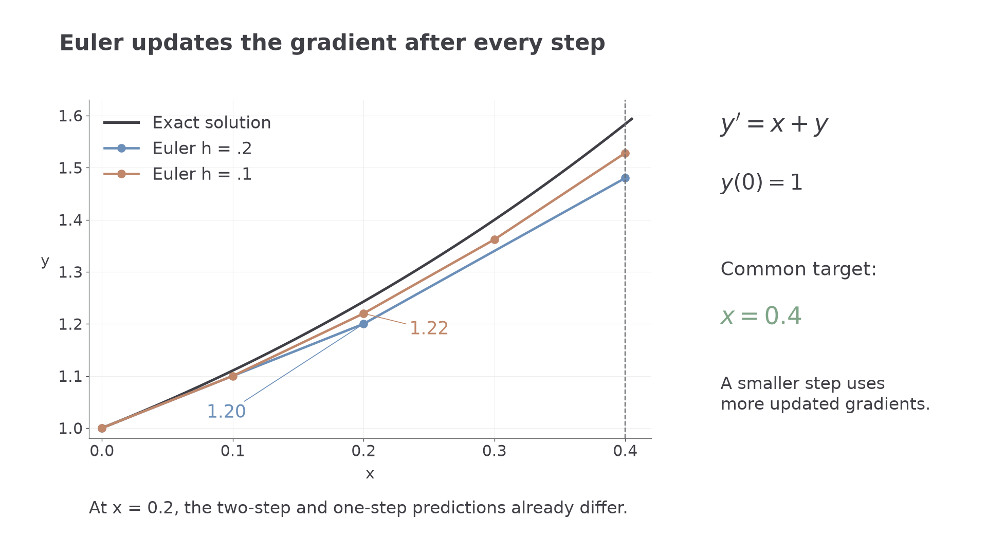
Check. At , two short steps give , whereas one long step gives . This answers the opening question: the intermediate gradient changes the prediction.
Euler's polygon follows straight pieces of successive tangents. It need not stay on the exact solution curve, even when the initial tangent is correct.
[DIAGRAM: asset_name: Euler steps and the exact solution; asset_slug: euler_step_comparison; caption: A new gradient after each step changes the polygonal path; description: The exact solution y=2 exp(x)-x-1 from (0,1) is plotted on x from 0 to 0.4 beside Euler polygons with h=0.2 and h=0.1. Nodes at x=0.2 have heights 1.20 and 1.22 and are labelled separately with clear leader lines. The common final target x=0.4 is marked.]
Watch out
Wrong: use in an Euler row, or lock the previous value with an absolute reference. Right: use both coordinates from the old row and let those references move down.
Halve the step once more for a shorter target.
Predict the endpoint, then average two gradients
Euler uses only the starting gradient. The modified Euler method used here also estimates the gradient at the end of the step, then averages the two. It is the explicit trapezium, or Heun, version of a second-order Runge–Kutta method.
Modified Euler method
For the current point , calculate
The are increments, already multiplied by . The endpoint in the calculation is an Euler prediction, not the final corrected value.
In the formula booklet.
Adapt the previous spreadsheet for . Keep the initial values and the two parameter cells, but replace the calculation columns and the update:
| Cell | New entry | Meaning |
|---|---|---|
| =\text{\H$1}(\text{A2}+\text{$H$2}\text{B2})$ | ||
| Predicted endpoint height | ||
| =\text{\H$1}((\text{A2}+\text{$H$1})+\text{$H$2}\text{D2})$ | ||
| =\text{A2}+\text{\H$1}$ | Next | |
| Corrected next |
Copy down, and copy down. There is no circular reference: the predicted height is calculated first, and the corrected height becomes the next row's starting value.
Worked example 3: two modified Euler steps
Question. Estimate for , , with .
Plan. At each step calculate the starting increment, the predicted endpoint increment, then their average.
Why this step? The second step starts from , not from the discarded Euler prediction .
Answer. .
Check. The exact value from is approximately . This modified Euler estimate is closer than the earlier Euler estimate at the same step length.
Change only to , as in the earlier Euler comparison.
Continue this lesson.
You’re previewing NovaLearn without an account. Create a free account to read the rest.
Create free account