SR11–SR15 - The Poisson distribution | OCR A-Level Further Mathematics B (MEI)

Model event counts in time or space and calculate their probabilities. SR11 and SR12 choose a suitable model, SR13 handles point and cumulative probabilities, and SR14 and SR15 connect the parameter to moments, interval lengths and independent totals.

Choose a Poisson model in context

A sensor counts flashes at an average of two per minute. Counting two independent minutes and simply doubling one minute's count both give expected count four. Why can the first be Poisson when the second is not?

You already know

A discrete distribution assigns probabilities to separate values. Independent means and variances add, but $\operatorname{Var}(2X)=4\operatorname{Var}(X)$ . A binomial count has a fixed number of trials and a constant success probability.

For counts such as faults along a cable or messages arriving during a fixed period, there may be no natural fixed number of trials. A Poisson model instead describes random events in a specified interval of time or space.

Poisson model

Write $X\sim\mathrm{Po}(\lambda)$ when $X$ has a Poisson distribution with parameter $\lambda$ , its expected count in the specified interval. Its possible values are $0,1,2,\ldots$ . A usual event-count model has $\lambda>0$ .

For a suitable model, events occur randomly, independently of one another and at a constant average rate over the interval being considered. Explain those statements in context. For messages, one message arriving must not trigger another, and the average arrival rate must remain steady through the period. A scheduled batch of messages or a sharp lunchtime surge would undermine these assumptions.

There can be two sensible models for the same setting. For a large number of independent components, each with a small failure probability, a binomial count may be natural. The rare failures may also behave like independent events at a steady average rate, suggesting a Poisson model. The qualitative link is useful for model choice; no fixed numerical thresholds are needed. Use the requested distribution when one is specified.

Do not replace a specified binomial calculation with a Poisson numerical approximation. Calculate binomial probabilities directly using the calculator. The link here concerns appropriate models.

Key idea

Choose the model from how events occur and what is counted. A Poisson parameter belongs to a stated interval, not just to the event's name.

Look for a failure of the process assumptions rather than a dislike of random variation itself.

Calculate an exact-count probability

Suppose calls arrive under a Poisson model with mean $3$ per ten-minute period. A count of three is not certain: the parameter is an average, and the whole probability function describes the variation around it.

Poisson probability function

For $X\sim\mathrm{Po}(\lambda)$ , with $\lambda>0$ ,

P(X=r)=e^{-\lambda}\frac{\lambda^r}{r!},\qquad r=0,1,2,\ldots

In particular, $P(X=0)=e^{-\lambda}$ , since $0!=1$ .

In the formula booklet.

Use the calculator's Poisson point-probability function with the parameter and required integer, or evaluate the supplied expression. Record the mathematical probability and parameter, rather than calculator button names.

Worked example 1: exactly three events

Question. Calls in a ten-minute period have distribution $X\sim\mathrm{Po}(3)$ . Find $P(X=3)$ .

Plan. Substitute the mean count and required count into the Poisson probability function.

\begin{aligned} P(X=3)&=e^{-3}\frac{3^3}{3!} &&\text{parameter and count are both }3\\ &=0.224041\ldots &&\text{evaluate} \end{aligned}

Why this step? The parameter is the mean for this ten-minute interval, not an event probability.

Answer. $P(X=3)=0.2240$ , to $4$ decimal places.

Check. A count at the mean is plausible, but its probability is well below one.

Change only the requested count to four. The parameter stays three because the interval and process have not changed.

Worked example 2: one more event

Question. For the same $X\sim\mathrm{Po}(3)$ , find $P(X=4)$ .

Plan. Keep the parameter fixed and change the factorial and power to the new count.

\begin{aligned} P(X=4)&=e^{-3}\frac{3^4}{4!} &&\text{new count, same mean}\\ &=0.168031\ldots &&\text{evaluate} \end{aligned}

Why this step? Replacing the parameter by four would describe a different model instead of a different outcome under the same model.

Answer. $P(X=4)=0.1680$ , to $4$ decimal places.

Check. Dividing the two formulae gives $P(X=4)/P(X=3)=3/4$ , agreeing with the calculated values.

Keep a few extra calculator digits for checks and later calculations; round the final probability only once.

Watch out

Wrong: $P(X=4)=e^{-4}4^4/4!$ when $X\sim\mathrm{Po}(3)$ . Changing the requested count does not change the mean parameter. Correct: $P(X=4)=e^{-3}3^4/4!$ .

Keep the model parameter fixed while changing the count below.

Translate cumulative events accurately

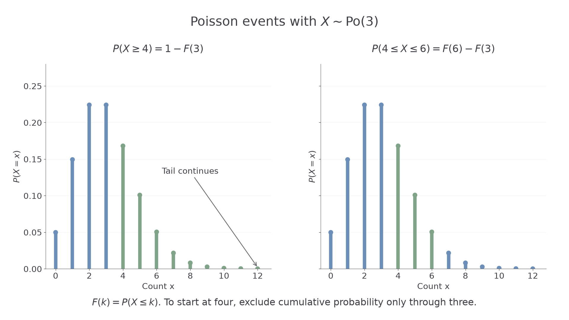
Let $F(k)=P(X\le k)$ , obtained from the calculator's cumulative Poisson function using the stated parameter. “At least four” starts at four, so its complement ends at three. A finite band is a difference of two cumulative probabilities.

Integer tails and bands

For integer bounds $a\le b$ on a non-negative integer-valued variable,

P(X\ge a)=1-F(a-1),\qquad P(a\le X\le b)=F(b)-F(a-1)

Take $F(-1)=0$ . A strict inequality must first be translated to its included integers.

Not in the formula booklet: learn it.

The same logic used for binomial tails applies, but the calculator parameters now describe a Poisson distribution.

[DIAGRAM: asset_name: Poisson tails and finite bands; asset_slug: poisson_tail_and_band; caption: Both events start at four, so both subtract the cumulative probability through three; description: Two exact Poisson probability graphs with parameter 3 share axes. The first highlights every value from four onwards for X at least four, with an arrow noting the continuing tail. The second highlights four, five and six only for the event four at most X at most six. Zero through three are blue in both panels.]
Both events start at four, so both subtract the cumulative probability through three

Worked example 3: an upper tail

Question. For $X\sim\mathrm{Po}(3)$ , determine $P(X\ge4)$ .

Plan. Complement the lower cumulative probability through three.

\begin{aligned} P(X\ge4)&=1-P(X\le3) &&\text{exclude }0,1,2,3\\ &=1-0.647231\ldots &&\text{cumulative output at }3\\ &=0.352768\ldots &&\text{remaining tail} \end{aligned}

Why this step? Subtracting $P(X\le4)$ would incorrectly remove the first included count.

Answer. $0.3528$ , to $4$ decimal places.

Check. This exceeds $P(X=4)=0.168031\ldots$ , since larger counts are also included.

Change only the upper end of the event: stop the included tail at six.

Worked example 4: a finite band

Question. For the same model, determine $P(4\le X\le6)$ .

Plan. Start with all counts through six and remove all counts below four.

\begin{aligned} P(4\le X\le6)&=P(X\le6)-P(X\le3) &&\text{remove the unwanted lower counts}\\ &=0.966491\ldots-0.647231\ldots &&\text{same parameter in both outputs}\\ &=0.319259\ldots &&\text{finite event} \end{aligned}

Why this step? Subtracting the cumulative probability through four would lose the probability at four as well.

Answer. $0.3193$ , to $4$ decimal places.

Check. It is below the full tail probability $0.352768\ldots$ ; the difference is the omitted probability above six.

Show the inequality before evaluating. This is particularly helpful when the words “fewer than”, “at most” and “more than” appear together.

Continue this lesson.

You’re previewing NovaLearn without an account. Create a free account to read the rest.

Create free account

Last Accessed

Core Pure

Mechanics (Major and Minor)

Statistics (Major and Minor)

Modelling with Algorithms

Numerical Methods

Extra Pure

Further Pure with Technology

SR11–SR15 - The Poisson distribution

Choose a Poisson model in context

Calculate an exact-count probability

Translate cumulative events accurately

Continue this lesson.

Learn faster with Nova