SR1–SR3 - Discrete distributions, mean and variance
Describe a finite random variable by its possible values and their probabilities. SR1 turns tables, formulae and graphs into probability statements; SR2 and SR3 use the same information to measure the distribution's centre and spread.
Build a valid probability function
A game awards only , or points. Can its expected score be , even though nobody can score that in one play? We will distinguish an average from a possible outcome.
You already know
Mutually exclusive probabilities add, the probabilities of all possible outcomes sum to , and . A random variable assigns a numerical value to each outcome of a random experiment.
For now the list of possible values is finite. A probability function can be a table, or an algebraic rule accompanied by the values on which it applies. The rule alone is incomplete: gives different distributions on different sets of values.
Discrete probability distribution
A discrete random variable takes separate possible values , with probabilities . Its probability function must satisfy for every value and . Probabilities at all other values are zero.
Use the total probability to find an unknown constant, then check that none of the resulting probabilities is negative. A list summing to can still be invalid if it contains a negative entry.
Worked example 1: normalise an algebraic rule
Question. The probability function is for , and zero otherwise. Determine and .
Plan. Make the three probabilities sum to one, then add the probabilities belonging to the event.
Why this step? The probability rule weights the values differently; there are three possible values, but they are not equally likely.
Answer. and .
Check. The probabilities are : all are non-negative and sum to .
Change only the greatest possible value from to . The normalising constant must change as well.
Worked example 2: extend the support
Question. Now for , and zero otherwise. Determine and .
Plan. Include the additional outcome when normalising and when finding the event probability.
Why this step? Keeping the old constant would make the total probability exceed one once the extra outcome was included.
Answer. and .
Check. .
The normalisation conditions are not listed as a separate formula in the booklet: learn them. They are also your first check on any table you construct.
Watch out
Wrong: still works after adding the value . The probabilities would sum to , not one. Correct: normalise the complete new support, giving and .
Check the total before using the next probability rule.
Read tables and probability graphs
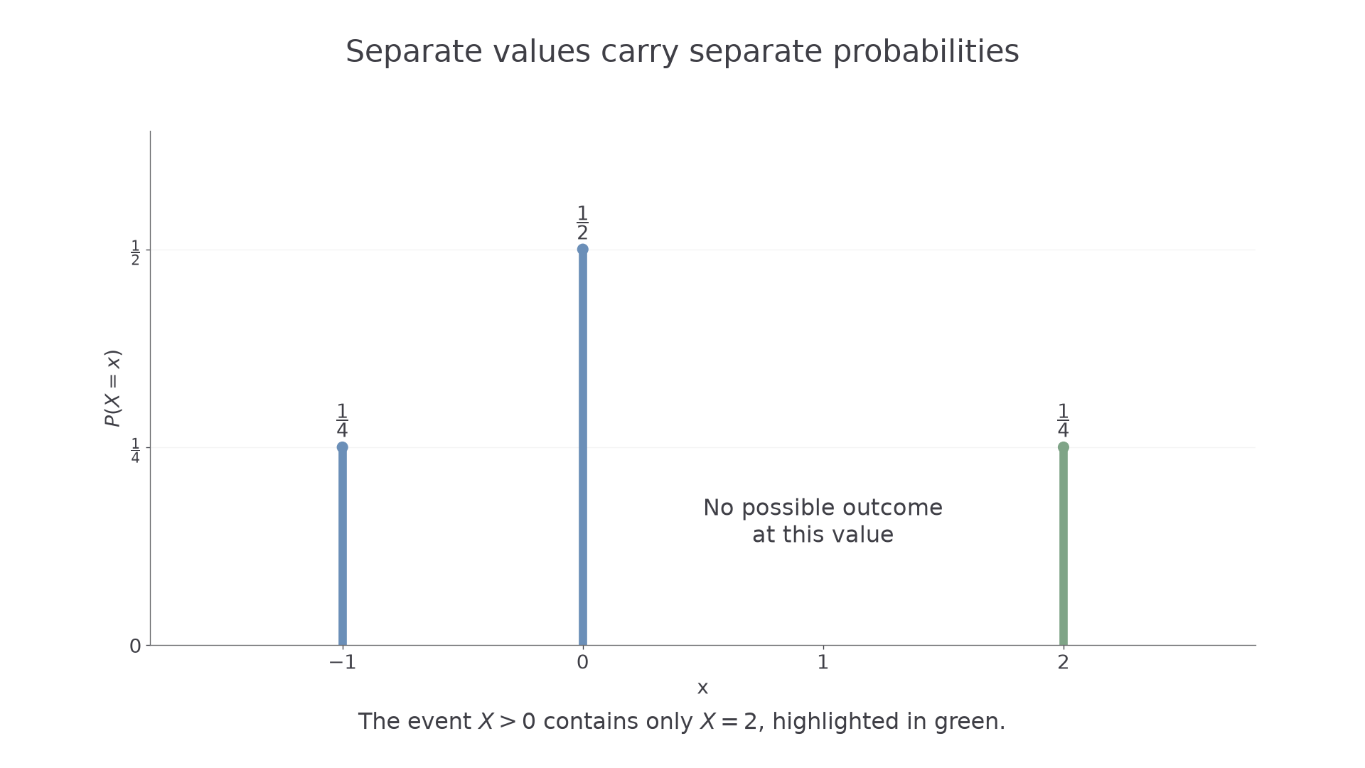
A probability graph places a separate bar or vertical line at each possible value. Its height is . Do not join the tops with a curve: values between the listed outcomes may be impossible.
Consider this distribution. Negative values can represent a loss or a signed change; probabilities themselves must still be non-negative.
[DIAGRAM: asset_name: A finite probability graph; asset_slug: drv_probability_graph; caption: Each height is a probability at one separate value, with no probability between the listed outcomes; description: A discrete probability graph has vertical lines at x minus one, zero and two with respective heights one quarter, one half and one quarter. The event X greater than zero highlights only the line at two. Both axes and all three probabilities are labelled.]
Worked example 3: a strict inequality
Question. For the table above, determine .
Plan. List the possible values that satisfy the inequality, then read their probabilities.
Why this step? Zero is a possible outcome with substantial probability, but a strict inequality excludes it.
Answer. .
Check. The excluded outcomes have total probability , leaving .
Change only the inequality to include its boundary. That adds the entire probability at zero.
Worked example 4: include the boundary
Question. For the same distribution, determine .
Plan. Include both zero and the positive outcome.
Why this step? In a discrete distribution, equality can carry positive probability, so changing the boundary can change the answer sharply.
Answer. .
Check. .
For discrete probability graphs, the heights sum to one. The width of a decorative bar has no probability meaning; the heights at the separate values are what you add.
Watch out
Wrong: . Equality includes the probability at zero, which is in this table. Correct: .
List the included values before drawing or adding the next probabilities.
Continue this lesson.
You’re previewing NovaLearn without an account. Create a free account to read the rest.
Create free account