Nc3, Nc4 - Midpoint, trapezium and Simpson's rules | OCR A-Level Further Mathematics B (MEI)

Nc3 approximates definite integrals using midpoint, trapezium and Simpson's rules, with the correct sample points and weights. Nc4 connects the rules, explains their usual orders and uses refinement output to assess accuracy. You will also use curvature to distinguish an estimate from a justified bound.

Choose midpoint heights or endpoint heights

For $\int_0^2x^2\,dx$ , one midpoint rectangle gives $2$ , while one trapezium gives $4$ . Their ordinary average, $3$ , is still wrong. Why does weighting the midpoint estimate twice as heavily give the exact answer $8/3$ ?

Start with the two simpler rules. Divide $[a,b]$ into $n$ equal strips, each of width $h=(b-a)/n$ . The midpoint rule samples once at the centre of each strip. The trapezium rule uses the two boundary heights of each strip.

You already know

A definite integral is a signed area. Keep stored precision through a calculation and round the reported output as requested. An approximation method's order describes how its error scales with step length; that is different from the order of convergence of a refinement sequence.

Write $x_j=a+jh$ and $y_j=f(x_j)$ . A midpoint height is $y_{j+1/2}=f(a+(j+1/2)h)$ , rather than an endpoint value.

Midpoint and trapezium rules

With $n$ equal strips and $h=(b-a)/n$ ,

M_n=h\sum_{j=0}^{n-1}f\left(a+\left(j+\frac12\right)h\right)

T_n=\frac h2\left(y_0+y_n+2\sum_{j=1}^{n-1}y_j\right)

$M_n$ uses $n$ midpoint values. $T_n$ uses $n+1$ endpoint values; interior endpoints receive weight $2$ because each belongs to two adjacent trapezia.

In the formula booklet.

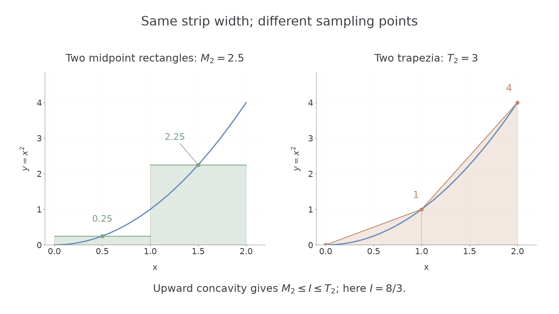
For a curve concave upwards throughout the interval, midpoint rectangles underestimate its integral and trapezia overestimate it: $M_n\le I\le T_n$ . For a curve concave downwards, the inequalities reverse. These curvature bounds are not printed separately in the booklet: learn them. They do not follow merely from the function being increasing.

[DIAGRAM: asset_name: Midpoint rectangles and trapezia on a convex curve; asset_slug: h645_b132_midpoint_trapezium; caption: For the upward-curving graph, the midpoint estimate is below the integral and the trapezium estimate is above it; description: Two panels show y equals x squared on zero to two, with two equal strips of width one. Sage midpoint rectangles use heights one quarter and nine quarters, giving M2 equal to 2.5. Clay trapezia use endpoint heights zero, one and four, giving T2 equal to three. The exact integral eight thirds is labelled in a separate strip.]
For the upward-curving graph, the midpoint estimate is below the integral and the trapezium estimate is above it

Worked example 1: two equal strips

Question. Approximate $I=\int_0^2x^2\,dx$ using $M_2$ and $T_2$ . Use the curve's shape to bound $I$ .

Plan. Calculate the common strip width, then use midpoint or endpoint samples as appropriate.

\begin{aligned} h&=\frac{2-0}{2}=1&&\text{two equal strips}\\ M_2&=1\left(0.5^2+1.5^2\right)=2.5&&\text{two midpoint heights}\\ T_2&=\frac12\left(0^2+2^2+2(1^2)\right)=3&&\text{three endpoint heights}\\ f''(x)&=2>0&&\text{concave upwards} \end{aligned}

Why this step? The midpoint samples are $0.5$ and $1.5$ , not $0$ , $1$ and $2$ . The two rules use different points even though the strip widths agree.

Answer. $M_2=2.5$ , $T_2=3$ , and $2.5\le I\le3$ .

Check. Direct integration gives $I=8/3$ , between the two approximations.

Change only the strip count from $2$ to $4$ . The interval and integrand stay fixed.

Worked example 2: halving the strip width

Question. Find $M_4$ and $T_4$ for the same integral, and update the bound.

Plan. Use width $0.5$ , with four midpoint samples and five endpoint samples.

\begin{aligned} h&=\frac24=0.5&&\text{refined width}\\ M_4&=0.5(0.25^2+0.75^2+1.25^2+1.75^2)&&\text{midpoints of the four strips}\\ &=2.625&&\text{weighted sum}\\ T_4&=\frac{0.5}{2}\left(0^2+2^2+2(0.5^2+1^2+1.5^2)\right)&&\text{endpoint rule}\\ &=2.75&&\text{weighted sum} \end{aligned}

Why this step? Halving the width doubles the number of strips, not the number of endpoint values: those change from $3$ to $5$ .

Answer. $M_4=2.625$ , $T_4=2.75$ , so $2.625\le I\le2.75$ .

Check. The bounding gap has fallen from $0.5$ to $0.125$ , a factor of $1/4$ .

A bounding interval can justify reported precision: if both endpoints round to the same value at the requested precision, every enclosed integral value does too. By contrast, similar-looking estimates without a known bound provide empirical evidence rather than a guarantee.

Watch out

Wrong: decide over- or under-estimation from whether the graph rises. Right: use its curvature. An increasing concave-down graph gives the opposite midpoint/trapezium ordering from an increasing concave-up graph.

Keep four strips and change only the integrand's power.

Simpson's rule uses an even number of subintervals

Simpson's rule combines values in successive triples, corresponding to a quadratic fitted across two equal subintervals. Adjacent triples share a boundary value.

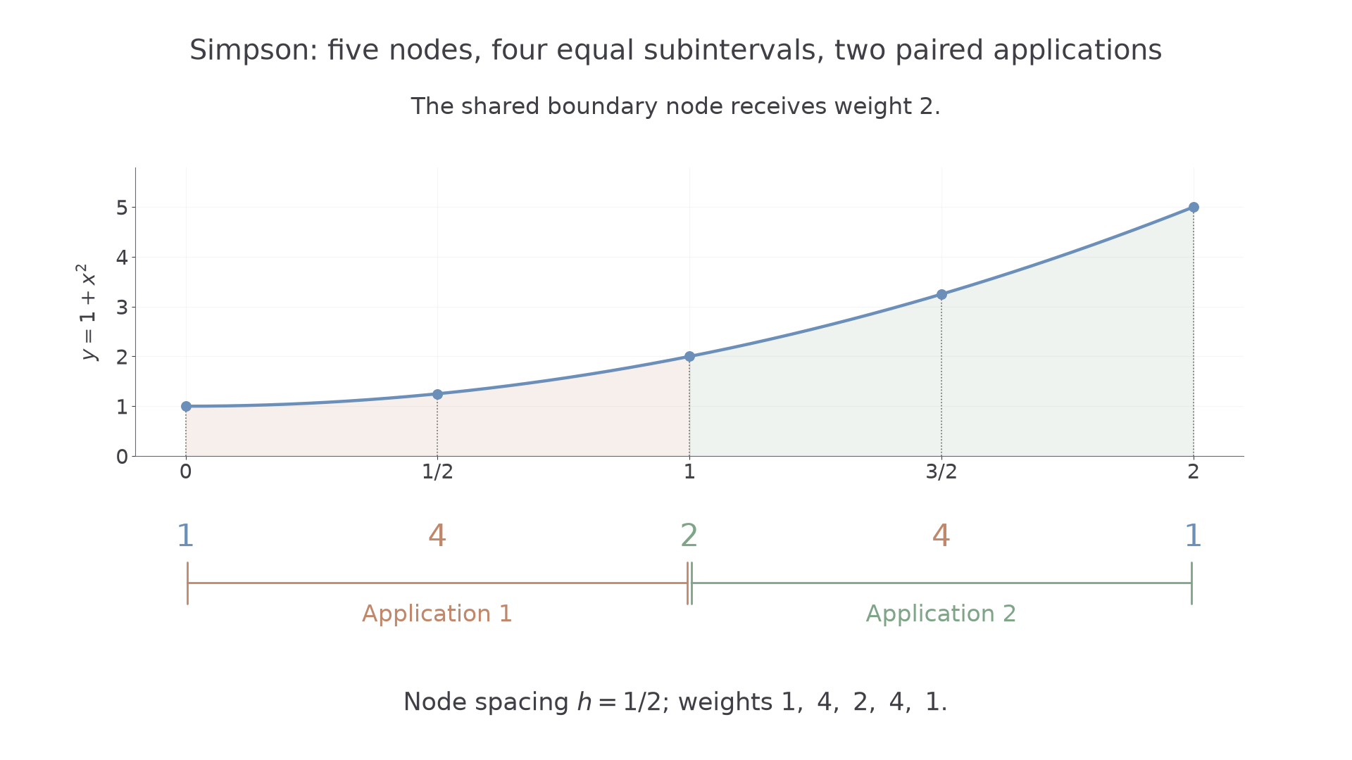
Use $S_{2n}$ for $2n$ equal subintervals, with $2n+1$ nodes. There are $n$ paired applications. We describe Simpson's rule by these nodes and applications, rather than by midpoint/trapezium “strips”.

Simpson's rule

For $2n$ equal subintervals, let $h=(b-a)/(2n)$ , with $y_j=f(a+jh)$ . Then

S_{2n}=\frac h3\left[ y_0+y_{2n} +4(y_1+y_3+\cdots+y_{2n-1}) +2(y_2+y_4+\cdots+y_{2n-2}) \right]

The weights are $1,4,2,4,\ldots,2,4,1$ . For one application, there are just three weights $1,4,1$ .

In the formula booklet.

The notation matters: in a worksheet row containing $M_n,T_n,S_{2n}$ , Simpson's node spacing is half the strip width used by the other two. Calculate the spacing from the formula you are actually applying.

[DIAGRAM: asset_name: Simpson nodes paired in triples; asset_slug: h645_b132_simpson_weights; caption: Four equal subintervals use five nodes with weights one four two four one; description: The graph of one plus x squared on zero to two has nodes at zero, one half, one, three halves and two. Two paired applications span zero to one and one to two, sharing the middle boundary node. A separate lower strip places weights one, four, two, four and one under the corresponding nodes, and marks the common node spacing one half.]
Four equal subintervals use five nodes with weights one four two four one

Worked example 3: five nodes, four subintervals

Question. Use Simpson's rule with node spacing $0.5$ to approximate $\int_0^2x^2\,dx$ .

Plan. There are four subintervals, so use $S_4$ and weights $1,4,2,4,1$ .

\begin{aligned} 2n&=\frac{2-0}{0.5}=4&&\text{count subintervals}\\ (y_0,y_1,y_2,y_3,y_4)&=(0,0.25,1,2.25,4)&&\text{evaluate at the nodes}\\ S_4&=\frac{0.5}{3}(0+4(0.25)+2(1)+4(2.25)+4)&&\text{apply the weights}\\ &=\frac{16}{6}=\frac83&&\text{simplify} \end{aligned}

Why this step? The factor outside is $h/3$ , with $h=0.5$ . Using the whole paired width $1$ would double the result.

Answer. $S_4=8/3$ .

Check. This equals the exact integral. Simpson's rule is exact for quadratic functions.

Change only the power from $2$ to $3$ , keeping the same interval and nodes.

Worked example 4: exactness extends to a cubic

Question. Apply the same Simpson calculation to $\int_0^2x^3\,dx$ .

Plan. Retain the spacing and weights, and update the function values.

\begin{aligned} (y_0,y_1,y_2,y_3,y_4)&=(0,0.125,1,3.375,8)&&\text{new node values}\\ S_4&=\frac{0.5}{3}(0+4(0.125)+2(1)+4(3.375)+8)&&\text{same Simpson weights}\\ &=\frac{24}{6}=4&&\text{evaluate} \end{aligned}

Why this step? The shared interior boundary at $x=1$ has weight $2$ ; the two intervening nodes have weight $4$ .

Answer. $S_4=4$ .

Check. The exact integral is $[x^4/4]_0^2=4$ . Simpson's rule is exact for cubics too, even though each local fitted curve is quadratic.

That cubic exactness is a useful surprise: local curve fitting can integrate a wider family exactly than the fitted degree alone suggests. For general functions, however, Simpson's rule is still an approximation. Its polynomial exactness through degree $3$ is not stated separately in the booklet; the calculations above demonstrate it for these examples.

Watch out

Wrong: use an odd number of equal subintervals with the standard composite Simpson formula, or assign weight $4$ to every interior node. Right: use an even count and alternate $4,2,\ldots,4$ .

Increase only the power again. Exactness is no longer automatic.

Combine existing estimates without new function values

The midpoint heights of a coarse grid become the new interior nodes when that grid is halved. This makes the rules fit together.

For example, coarse nodes $a,a+h,a+2h$ and their intervening midpoints together form a grid of spacing $h/2$ . Combining old endpoint and midpoint sums can therefore produce the refined trapezium and Simpson approximations.

Continue this lesson.

You’re previewing NovaLearn without an account. Create a free account to read the rest.

Create free account

Last Accessed

Core Pure

Mechanics (Major and Minor)

Statistics (Major and Minor)

Modelling with Algorithms

Numerical Methods

Extra Pure

Further Pure with Technology

Nc3, Nc4 - Midpoint, trapezium and Simpson's rules

Choose midpoint heights or endpoint heights

Simpson's rule uses an even number of subintervals

Combine existing estimates without new function values

Continue this lesson.

Learn faster with Nova