Nc1, Nc2 - Forward and central difference methods | OCR A-Level Further Mathematics B (MEI)

Estimate a derivative from a function or a table using forward and central differences. Choose the points and step length carefully, recognise first- and second-order behaviour in numerical output, and explain why decreasing the step eventually becomes unhelpful in limited precision.

Estimate a gradient from the point ahead

You want the gradient of $y=e^x$ at $x=1$ . A numerical calculation with step $0.01$ gives a useful answer close to $2.7183$ . With a much smaller step, $10^{-7}$ , the same calculation can give zero. How can moving the points closer together destroy the answer?

First separate the geometry from the machine arithmetic. Consider the exact values below for $f(x)=x^3$ . We want the gradient at $x=1$ , but can start by measuring the rise between two nearby points.

$x$	$1$	$1.05$	$1.1$	$1.2$
$f(x)$	$1$	$1.157625$	$1.331$	$1.728$

You already know

A derivative is a tangent gradient, and the gradient between two points is change in $y$ divided by change in $x$ . Rounding stored values can lose information, especially when nearly equal numbers are subtracted. The order of a step-length method describes how its error depends on the step, rather than merely how many digits appear on screen.

A chord gives an average gradient over an interval. A forward difference uses the target point and a point to its right. For a smooth curve and a sufficiently small step, this chord gradient estimates the tangent gradient at the target.

Forward difference estimate

For a positive step $h$ , with both function values available,

F(h)=\frac{f(x+h)-f(x)}{h}\approx f'(x)

The denominator is the actual separation of the two inputs. The estimate is useful when the function behaves smoothly near the target and the input values have adequate accuracy.

Not in the formula booklet: learn it.

If the function is supplied, evaluate it at the required inputs. If only data are supplied, use available inputs: a smaller step is not a licence to invent an intermediate function value.

Worked example 1: a forward step from an endpoint

Question. Use the table above to estimate $f'(1)$ by the forward difference method with $h=0.2$ .

Plan. Select the target value and the value $0.2$ to its right, then divide their change by $0.2$ .

\begin{aligned} x+h&=1.2&&\text{point ahead of the target}\\ f(1.2)-f(1)&=1.728-1=0.728&&\text{vertical change}\\ F(0.2)&=\frac{0.728}{0.2}=3.64&&\text{chord gradient} \end{aligned}

Why this step? The derivative is being estimated at $1$ ; the forward chord must start there, rather than join two other convenient table entries.

Answer. $f'(1)\approx3.64$ .

Check. Differentiating the supplied function gives $f'(1)=3$ . The curve becomes steeper to the right, so a forward average larger than $3$ makes sense.

Change only the step length, from $0.2$ to $0.1$ . The target and function stay fixed, so the two estimates can be compared fairly.

Worked example 2: halve the forward step

Question. Use $h=0.1$ to estimate the same derivative by the forward difference method.

Plan. Keep the target value and replace the right-hand value by the one at $1.1$ .

\begin{aligned} x+h&=1.1&&\text{new right-hand input}\\ f(1.1)-f(1)&=1.331-1=0.331&&\text{new rise}\\ F(0.1)&=\frac{0.331}{0.1}=3.31&&\text{divide by the new step}\\ |3.31-3|&=0.31<0.64&&\text{compare absolute errors} \end{aligned}

Why this step? Changing the numerator without changing the denominator would no longer calculate the gradient between the selected points.

Answer. $f'(1)\approx3.31$ , closer to the reference value than $3.64$ .

Check. The estimate is still above $3$ , but is nearer to the tangent gradient as the chord shortens.

At an endpoint of a data set, a forward estimate may be possible even though a central estimate is unavailable.

Watch out

Wrong: divide $f(1.1)-f(1)$ by $1.1$ . Right: divide by $1.1-1=0.1$ . The denominator is a change in input, not the input itself.

Use a shorter interval in a fresh two-point data set.

Balance the gradient estimate about the target

A forward chord lies wholly to one side of the target. A central chord uses points on opposite sides, which usually balances much of that one-sided error. Its gradient need not be the gradient at either endpoint.

[DIAGRAM: asset_name: Forward and central chords beside the same tangent; asset_slug: h645_b131_chord_geometry; caption: Both panels use x equal to 1 and h equal to 0.4. The central chord is much closer to parallel with the tangent; description: Two plots of y equals x cubed show the tangent at the target one comma one in sage. The forward panel joins one comma one to one point four comma two point seven four four in blue and labels gradient 4.36. The central panel joins zero point six comma zero point two one six to one point four comma two point seven four four in clay and labels gradient 3.16. Both show the tangent gradient 3 and labelled horizontal spans h or 2h. The central chord does not pass through the target point.]
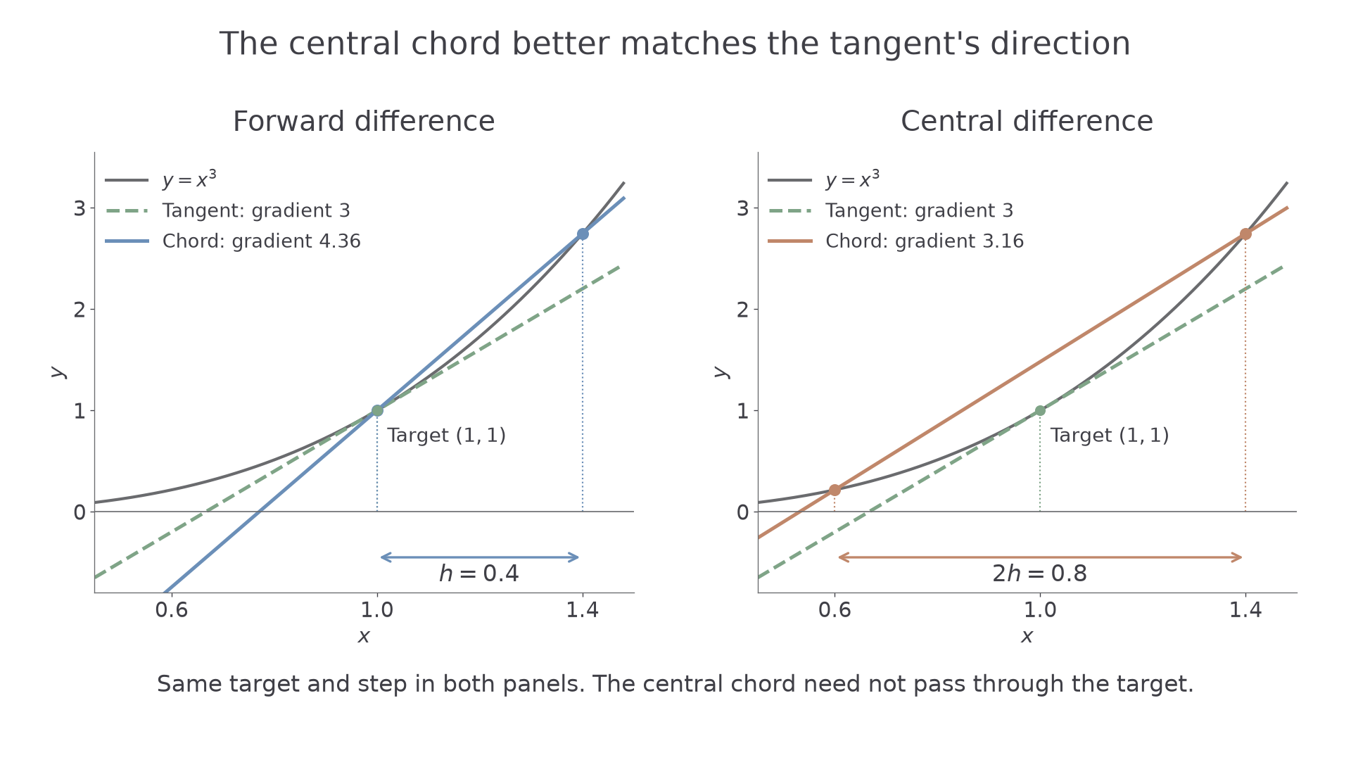
Both panels use x equal to 1 and h equal to 0.4. The central chord is much closer to parallel with the tangent

The central chord spans twice the step length. This is the reason for the $2h$ in its denominator.

Central difference estimate

For a positive step $h$ , with both values available at equal distances from the target,

C(h)=\frac{f(x+h)-f(x-h)}{2h}\approx f'(x)

The target is the midpoint of the two inputs. As with forward differences, useful accuracy depends on smooth behaviour near the target and sufficiently accurate function values.

Not in the formula booklet: learn it.

The following exact cubic values let us compare forward and central estimates at the same target with the same $h$ .

$x$	$0.8$	$0.9$	$0.95$	$1$	$1.05$	$1.1$	$1.2$
$f(x)=x^3$	$0.512$	$0.729$	$0.857375$	$1$	$1.157625$	$1.331$	$1.728$

Worked example 3: use a symmetric pair

Question. Estimate $f'(1)$ by the central difference method with $h=0.2$ . Compare its error with the forward estimate $3.64$ .

Plan. Use the values at $0.8$ and $1.2$ , then compare both estimates with the exact gradient $3$ .

\begin{aligned} x-h&=0.8,\qquad x+h=1.2&&\text{equal offsets from the target}\\ C(0.2)&=\frac{1.728-0.512}{2(0.2)} =\frac{1.216}{0.4}=3.04&&\text{whole chord width}\\ |C(0.2)-3|&=0.04&&\text{central absolute error}\\ |3.64-3|&=0.64&&\text{forward absolute error} \end{aligned}

Why this step? The numerator uses the right and left points, not the right and target points. Its denominator must cover the same interval.

Answer. $f'(1)\approx3.04$ . Its absolute error is $0.04$ , compared with $0.64$ for the forward estimate.

Check. The input separation is $1.2-0.8=0.4$ . The answer is close to the known tangent gradient.

Change only $h$ to $0.1$ . Both endpoints move towards the same target by the same amount.

Worked example 4: halve the central step

Question. Estimate $f'(1)$ centrally with $h=0.1$ , and compare its error with the preceding central estimate.

Plan. Select the symmetric pair $0.9,1.1$ and divide by their separation.

\begin{aligned} C(0.1)&=\frac{1.331-0.729}{2(0.1)} &&\text{use the symmetric pair}\\ &=\frac{0.602}{0.2}=3.01&&\text{calculate the gradient}\\ |3.01-3|&=0.01=\frac{0.04}{4}&&\text{error is quartered} \end{aligned}

Why this step? A central step of $0.1$ means a total chord width of $0.2$ . Confusing those two lengths would double the answer.

Answer. $f'(1)\approx3.01$ , with absolute error $0.01$ .

Check. Both central estimates overestimate $3$ , and shortening the chord has reduced the discrepancy.

With a supplied function defined on both sides, you can evaluate a new symmetric pair. With a table alone, you need a symmetric pair already in that table. At its left endpoint there may be no such pair; at its right endpoint even a forward estimate may be unavailable. These are limitations of the supplied data, not evidence that the derivative fails to exist.

Watch out

Wrong: use the two nearest entries if they are at different distances from the target, and call their chord gradient a central estimate there. Right: check that the target is their midpoint before using the central formula.

Compare another central estimate with a supplied forward result.

Read the order from changing errors or differences

One successful step reduction does not establish a general pattern. Use a sequence of step lengths, keep the target fixed, and examine what happens as the step shrinks. Work with retained values, rather than repeatedly rounding the displayed output.

Order of a difference method

A method has order $p$ when, in the small-step range where its leading step-length error dominates, the magnitude of that error is approximately proportional to $h^p$ . The forward difference method is generally first order; the central difference method is generally second order.

“Generally” matters: a particular function or target can make an error term vanish. Poorly resolved or insufficiently smooth functions need not show the usual pattern.

This statement concerns the error caused by replacing a tangent by a finite chord. It assumes arithmetic errors are small enough not to hide that pattern.

Step reduction and empirical order

If the step-length error is approximately proportional to $h^p$ , reducing $h$ by a factor $k>1$ multiplies its magnitude approximately by

\frac1{k^p}

In particular, halving $h$ usually halves the forward error and quarters the central error.

Not in the formula booklet: learn it.

You are identifying an observed rate, rather than proving the order. For this investigation, the exact derivative of $e^x$ at $1$ is $e=2.718281828459\ldots$ . The table displays ten decimal places; calculations retain more digits.

Worked example 5: a known reference reveals the errors

Question. The table gives estimates of the derivative of $e^x$ at $1$ , with their absolute errors. What order does each column suggest?

$h$	$F(h)$	Forward error	$C(h)$	Central error
$0.2$	$3.0091754714$	$0.2908936429$	$2.7364399856$	$0.0181581572$
$0.1$	$2.8588419549$	$0.1405601264$	$2.7228145639$	$0.0045327355$
$0.05$	$2.7873857921$	$0.0691039636$	$2.7194145875$	$0.0011327590$
$0.025$	$2.7525452843$	$0.0342634558$	$2.7185649917$	$0.0002831632$
$0.0125$	$2.7353421002$	$0.0170602718$	$2.7183526176$	$0.0000707891$

Plan. Divide each new error by the previous error and relate the limiting ratios to the halved steps.

\begin{aligned} \text{forward ratios}&\approx0.483201,\ 0.491633,\ 0.495825,\ 0.497915 &&\text{approach }1/2\\ \text{central ratios}&\approx0.249625,\ 0.249906,\ 0.249977,\ 0.249994 &&\text{approach }1/4\\ 1/2&=(1/2)^1&&\text{first-order forward method}\\ 1/4&=(1/2)^2&&\text{second-order central method} \end{aligned}

Why this step? A ratio has meaning only alongside the change in $h$ . Quartering an error when $h$ is halved indicates a different order from quartering it when $h$ is quartered.

Answer. The evidence suggests order $1$ for forward differences and order $2$ for central differences, in agreement with their usual behaviour.

Check. At every displayed step, the central error is smaller; its error also falls faster as $h$ is reduced.

Change only the availability of the reference derivative. Suppose the central output is known, but the exact derivative is not. Consecutive changes can still reveal an order when one leading error term dominates.

Continue this lesson.

You’re previewing NovaLearn without an account. Create a free account to read the rest.

Create free account

Last Accessed

Core Pure

Mechanics (Major and Minor)

Statistics (Major and Minor)

Modelling with Algorithms

Numerical Methods

Extra Pure

Further Pure with Technology

Nc1, Nc2 - Forward and central difference methods

Estimate a gradient from the point ahead

Balance the gradient estimate about the target

Read the order from changing errors or differences

Continue this lesson.

Learn faster with Nova