Tc1, Tc2, Tc4–Tc6 - Software solutions and tangent fields | OCR A-Level Further Mathematics B (MEI)

Explore first-order differential equations with a computer algebra system and a tangent-field plotter. You will control parameters, select and verify particular solutions, use isoclines to sketch a field, and read the domain and shape of a solution from its local directions.

Control the equation and its solution family separately

For $dy/dx=x-y$ , every point on the line $y=x$ has gradient zero. Does that make $y=x$ a solution?

A tangent field lets you see the trap: a line joining points with the same required gradient need not have that gradient itself. First, obtain some actual solution curves to compare with the field.

You already know

A first-order general solution contains a free constant. An initial condition selects a particular solution. You already know the integrating-factor method; here software performs the analytical solving while you interpret and check its output.

Use a CAS differential-equation solver with independent variable $x$ and dependent function $y(x)$ . Enter the equation, request a general analytical solution and record any restrictions. Exact algebraic output is different from a table of numerical approximations. Some equations have no elementary analytical solution, so a failed symbolic request does not imply that no solution curve exists.

Consider

\frac{dy}{dx}=x-y+a

where $a$ changes the equation. The CAS can return

y=x+a-1+Ce^{-x}

with arbitrary real $C$ . This family, and the software procedures below, are not printed in the formula booklet.

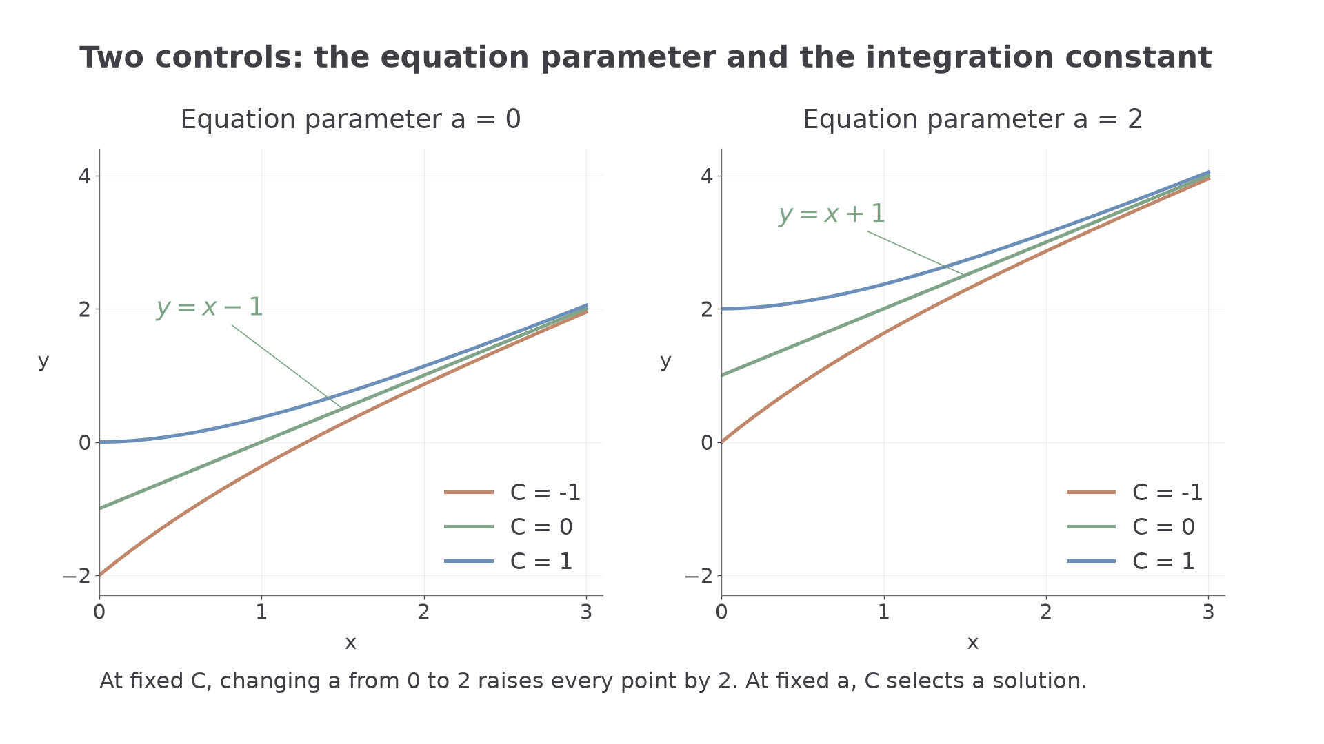
Plot this expression with separate sliders for $a$ and $C$ . Keep one fixed while varying the other. Different CAS systems may call the arbitrary constant something else; its mathematical role is unchanged.

Worked example 1: vary the integration constant

Question. Use analytical software to find the family for $y'=x-y$ , then describe the curves with $C=-1,0,1$ .

Plan. Set the equation parameter to zero, obtain the general family and vary only its integration constant.

Software request or setting	Exact result or interpretation
Solve $y'+y=x$ for $y(x)$	$y=x-1+Ce^{-x}$
Set $a=0$ ; vary $C=-1,0,1$	Three solutions of the same equation
Evaluate at $x=0$	$y(0)=C-1$ , giving $-2,-1,0$
Set $C=0$	Straight-line solution $y=x-1$

Why this step? Varying $C$ selects solutions of one equation; it does not alter the differential equation.

Answer. The family is $y=x-1+Ce^{-x}$ . The selected curves have initial heights $-2,-1,0$ .

Check. Differentiating the family gives $1-Ce^{-x}$ , and $x-y=1-Ce^{-x}$ , so every plotted member satisfies the equation.

Change only the equation parameter from $a=0$ to $a=2$ ; retain the same three slider values of $C$ .

Worked example 2: vary the equation parameter

Question. Obtain the analytical family for $y'=x-y+2$ , and compare those three curves with example 1.

Plan. Change the CAS equation as well as the plot's parameter, then inspect the new family.

Software request or setting	Exact result or interpretation
Solve $y'+y=x+2$ for $y(x)$	$y=x+1+Ce^{-x}$
Set $a=2$ ; vary $C=-1,0,1$	Solutions of the new equation
Evaluate at $x=0$	$y(0)=C+1$ , giving $0,1,2$
Compare at the same $C$	Each curve is $2$ units higher

Why this step? Changing $a$ changes the whole family. Reusing a plot with the old equation would investigate the wrong differential equation.

Answer. The family is $y=x+1+Ce^{-x}$ , translated upwards by $2$ at fixed $C$ .

Check. $y'=1-Ce^{-x}=x-y+2$ , with no restriction on real $x$ .

For either fixed $a$ , distinct values of $C$ give a difference $(C_1-C_2)e^{-x}$ , which never vanishes. These particular family members cannot cross.

[DIAGRAM: asset_name: Equation and integration-constant sliders; asset_slug: cas_family_parameters; caption: Changing C selects a curve, while changing a changes the differential equation; description: Two panels plot exact members y=x+a-1+C exp(-x) for a=0 and a=2, using C=-1,0,1 with matched colours. The two panels use matching axis ranges. The C=0 straight-line solution is labelled in each panel; an annotation states the two-unit vertical change at fixed C.]
Changing C selects a curve, while changing a changes the differential equation

Watch out

Wrong: set the arbitrary constant to zero because the software has returned a general solution. Right: retain it, label the parameter you are changing and apply an initial condition only when one is supplied.

Change the equation parameter again.

Verify both the equation and the initial condition

A verification has two separate targets: the proposed function must satisfy the differential equation throughout its stated interval, and it must satisfy the given condition. Checking one numerical point cannot establish the differential identity.

For a candidate $y=Y(x)$ , calculate $Y'(x)$ and independently calculate $f(x,Y(x))$ . Show that they agree, then check the initial condition. A CAS can differentiate and simplify the residual $Y'-f(x,Y)$ to zero. Record the expressions being compared, rather than only “software says true”. This verification procedure is not supplied in the booklet.

Worked example 3: select one family member

Question. For $a=0$ , use the family $y=x+a-1+Ce^{-x}$ to find the solution through $(0,2)$ , then verify it.

Plan. Determine $C$ , differentiate the selected function and substitute it into the right side independently.

\begin{aligned} 2&=-1+C\implies C=3 && \text{apply the initial condition}\\ Y(x)&=x-1+3e^{-x} && \text{select the member}\\ Y'(x)&=1-3e^{-x} && \text{differentiate}\\ x-Y(x)&=x-(x-1+3e^{-x})=1-3e^{-x} && \text{substitute separately} \end{aligned}

Why this step? Agreement of these expressions verifies the equation for every real $x$ , rather than merely at the starting point.

Answer. $y=x-1+3e^{-x}$ , for real $x$ .

Check. $Y(0)=-1+3=2$ . Both the equation and the initial condition hold.

Change only $a$ to $2$ , keeping the same initial condition.

Worked example 4: a family of particular solutions

Question. Select and verify the solution for $a=2$ through $(0,2)$ . Explain how the integration constant has changed.

Plan. Apply the unchanged point to the new equation's family, then check both requirements.

\begin{aligned} 2&=1+C\implies C=1 && \text{new family, same point}\\ Y(x)&=x+1+e^{-x} && \text{particular solution}\\ Y'(x)&=1-e^{-x} && \text{differentiate}\\ x-Y(x)+2&=x-(x+1+e^{-x})+2=1-e^{-x} && \text{verify the equation} \end{aligned}

Why this step? Keeping the initial point fixed does not keep $C$ fixed when the equation changes.

Answer. $y=x+1+e^{-x}$ , for real $x$ ; the constant is now $1$ , rather than $3$ .

Check. $Y(0)=2$ . More generally, the initial condition gives $C=3-a$ , producing the family of particular solutions

y=x+a-1+(3-a)e^{-x}

with the same starting point and varying $a$ .

At $a=3$ , this family contains the straight line $y=x+2$ . Sliders can reveal such a special case, but substitution explains why it works.

Watch out

Wrong: verify only $Y(0)=2$ , or compare $Y'$ with the unspecialised expression $x-y+a$ . Right: substitute the candidate for every occurrence of $y$ , simplify, and also check the condition.

Use one new equation parameter with the same point.

Continue this lesson.

You’re previewing NovaLearn without an account. Create a free account to read the rest.

Create free account

Last Accessed

Core Pure

Mechanics (Major and Minor)

Statistics (Major and Minor)

Modelling with Algorithms

Numerical Methods

Extra Pure

Further Pure with Technology

Tc1, Tc2, Tc4–Tc6 - Software solutions and tangent fields

Control the equation and its solution family separately

Verify both the equation and the initial condition

Continue this lesson.

Learn faster with Nova