Sb4–Sb7 - Pearson's product moment correlation | OCR A-Level Further Mathematics B (MEI)

Calculate Pearson's product moment correlation coefficient and use a valid population test, with either critical values or software output. You will also interpret the size of a correlation, which answers a different question from statistical significance.

Calculating the pmcc

If you convert one variable from seconds into hundredths of a second, should its correlation with another variable become one hundred times larger?

No. Correlation measures how the variables vary together relative to their own spreads. A change of units scales both parts of that comparison.

You already know

A scatter diagram reveals direction, curvature and outliers. Keep raw observations paired. Pearson's coefficient describes a linear relationship; a curved relationship can have zero pmcc.

Use $r$ for a sample coefficient and $\rho$ for the population correlation. They are different quantities: the sample provides evidence about the population.

Centred sums and Pearson's coefficient

For $n$ paired observations, with nonzero variation in both variables:

\begin{aligned} S_{xx}&=\sum x_i^2-\frac{(\sum x_i)^2}{n}\\ S_{yy}&=\sum y_i^2-\frac{(\sum y_i)^2}{n}\\ S_{xy}&=\sum x_iy_i-\frac{(\sum x_i)(\sum y_i)}{n}\\ r&=\frac{S_{xy}}{\sqrt{S_{xx}S_{yy}}} \end{aligned}

Here $-1\le r\le1$ . If either variable is constant, the denominator is zero and $r$ is undefined.

In the formula booklet.

For raw data, enter the two columns in paired-variable statistics mode and obtain $r$ from the calculator. Check the number of pairs and the sign against the scatter diagram. From summary statistics, show the centred sums and substitution.

Worked example 1: raw paired data

Question. Five randomly sampled devices have response times $x$ and $y$ , in seconds, under two operating conditions:

Device	$A$	$B$	$C$	$D$	$E$
$x$	$1$	$2$	$3$	$4$	$5$
$y$	$2$	$4$	$5$	$4$	$7$

Calculate the pmcc.

Plan. Enter paired columns into the calculator; use the centred sums to check the resulting coefficient.

\begin{aligned} \sum x&=15,\quad \sum y=22&&\text{paired-column totals}\\ S_{xx}&=55-\frac{15^2}{5}=10&&\text{centre the }x\text{ values}\\ S_{yy}&=110-\frac{22^2}{5}=13.2&&\text{centre the }y\text{ values}\\ S_{xy}&=76-\frac{15(22)}5=10&&\text{centre the cross-products}\\ r&=\frac{10}{\sqrt{10(13.2)}}=0.870388\ldots&&\text{standardise} \end{aligned}

Why this step? The divisor is the geometric mean of the two centred sums of squares, not their product alone.

Answer. $r=0.870$ to $3$ significant figures.

Check. The value lies between $-1$ and $1$ , and its positive sign agrees with the broad increasing pattern.

Change only the units of $x$ : multiply each $x$ value by $100$ , calling the new variable $u$ .

Worked example 2: summary statistics after a unit change

Question. The same data expressed using $u=100x$ have

\begin{gathered} n=5,\quad \sum u=1500,\quad \sum y=22\\ \sum u^2=550000,\quad \sum y^2=110,\quad \sum uy=7600 \end{gathered}

Calculate the correlation between $u$ and $y$ .

Plan. Recalculate the centred sums in the new units, then compare their scaling in the quotient.

\begin{aligned} S_{uu}&=550000-\frac{1500^2}{5}=100000&&\text{squared units scale by }100^2\\ S_{yy}&=13.2&&\text{unchanged variable}\\ S_{uy}&=7600-\frac{1500(22)}5=1000&&\text{cross-products scale by }100\\ r&=\frac{1000}{\sqrt{100000(13.2)}}&&\text{same coefficient formula}\\ &=0.870388\ldots&&\text{scale factors cancel} \end{aligned}

Why this step? The factor $100$ in the numerator is cancelled by $\sqrt{100^2}$ in the denominator.

Answer. The correlation remains $0.870$ .

Check. Both descriptions contain the same paired information. A unit change cannot strengthen its linear pattern.

Adding a constant also leaves centred deviations unchanged. Positive changes of scale and origin preserve $r$ ; reversing one axis by multiplying it by a negative number reverses its sign.

Watch out

Wrong: divide $S_{xy}$ by $S_{xx}S_{yy}$ without a square root, or use $n-1$ in these centred-sum formulae. Right: use the displayed expressions consistently.

Try a fresh set of summary statistics.

When a Pearson test is appropriate

Calculating a coefficient is not the same as justifying a hypothesis test. The reference probabilities for a Pearson test rely on a population model.

The Pearson-test setting

The data must be random on random, with both variables random, and modelled as drawn from a bivariate Normal distribution. A roughly elliptical scatter cloud can support that assumption; it cannot prove it.

A curved cloud, strong skewness, two distinct clusters or a conspicuous outlier can make this model implausible. The formal density of the bivariate Normal distribution is not needed: inspect the shape and consider how the observations arose.

[DIAGRAM: asset_name: A plausible population model is more than a straight trend; asset_slug: pearson_assumption_clouds; caption: An approximately elliptical cloud supports a bivariate Normal model; a strongly curved cloud raises doubts; description: Two scatter panels have identical axis labels X and Y. The left contains a roughly elliptical tilted blue cloud, labelled both variables sampled and bivariate Normal plausible. The right contains a curved monotonic blue cloud, labelled linear Normal-cloud model doubtful. No hypothesis-test result is inferred solely from either diagram.]
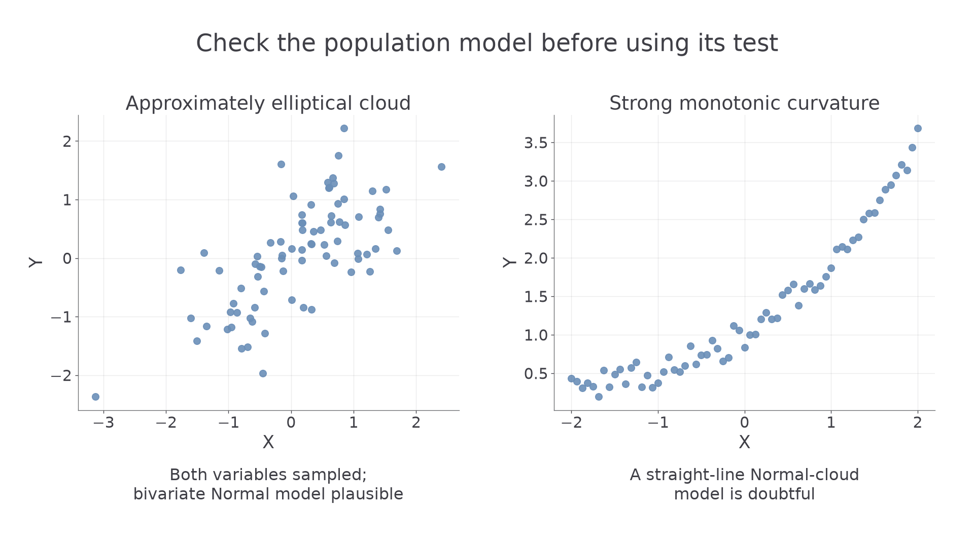
An approximately elliptical cloud supports a bivariate Normal model

A random sample and random-on-random data are separate requirements. Random sampling concerns how observational units are selected; random on random concerns whether both measurements vary randomly. Randomly choosing experimental runs does not make pre-set input values random.

For controlled loads and measured spring extensions, use the random-on-non-random regression model later in this section. This Pearson population test is not appropriate because the controlled variable has no population distribution of the required kind.

Key idea

Justify both the data structure and the distributional model; “the points look correlated” is not enough.

Choose the case that meets both conditions.

Tests using critical values

Choose the alternative from the research question before looking at the sample coefficient. A question about any correlation needs two tails; a pre-specified positive or negative direction needs one.

Pearson hypotheses

For population correlation $\rho$ , the null hypothesis is $\mathrm{H_0}:\rho=0$ . Alternatives are $\rho>0$ , $\rho<0$ or $\rho\ne0$ . Define the population and variables in context; do not write hypotheses about the observed sample value $r$ .

Use the booklet table's row $n$ , the number of pairs, and the correct one-tail or two-tail heading. The same columns carry different significance levels:

$n=12$ , Pearson table	One-sided $5\%$	Two-sided $5\%$
Critical magnitude	$0.4973$	$0.5760$

For a positive alternative, reject for sufficiently large positive $r$ ; for a negative alternative, use the negative critical value. For a two-sided alternative, compare $|r|$ with the critical magnitude. These table values are in the formula booklet.

Worked example 3: a pre-specified positive alternative

Question. A random sample of $12$ adults gives $r=0.55$ between height and hand span. Assume a bivariate Normal population. Test at $5\%$ for positive correlation.

Plan. State population hypotheses, use the one-sided critical value, then give a cautious contextual conclusion.

\begin{aligned} \mathrm{H_0}&:\rho=0&&\text{no population correlation}\\ \mathrm{H_1}&:\rho>0&&\text{positive population correlation}\\ r_{\mathrm{crit}}&=0.4973&&n=12,\text{ one-sided }5\%\\ 0.55&>0.4973&&\text{inside the rejection region} \end{aligned}

Here $\rho$ is the population correlation between adult height and hand span.

Why this step? “Positive” specifies the upper tail. Using the two-sided column would answer a different research question.

Answer. Reject $\mathrm{H_0}$ . There is sufficient evidence at $5\%$ to suggest positive correlation between height and hand span in the adult population sampled.

Check. The coefficient has the direction specified by the alternative, and the comparison uses $12$ pairs rather than a degrees-of-freedom row.

Continue this lesson.

You’re previewing NovaLearn without an account. Create a free account to read the rest.

Create free account

Last Accessed

Core Pure

Mechanics (Major and Minor)

Statistics (Major and Minor)

Modelling with Algorithms

Numerical Methods

Extra Pure

Further Pure with Technology

Sb4–Sb7 - Pearson's product moment correlation

Calculating the pmcc

When a Pearson test is appropriate

Tests using critical values

Continue this lesson.

Learn faster with Nova