TC1–TC5 - Families of curves with software | OCR A-Level Further Mathematics B (MEI)

Investigate cartesian, polar and parametric families using sliders and CAS. Turn observations into checked general statements, describe the curves precisely, and convert their equations without losing domains, branches or exceptional points.

A slider suggests a pattern; algebra checks it

A graph plotter draws two branches of

y=\frac{x^2+a}{x+1}

For one slider value, the branches seem to become a straight line. Has a whole curve really changed into a complete line, or is the picture hiding something?

Start with a fixed plotting window, say $-5\le x\le5$ , $-6\le y\le6$ , and a slider $-2\le a\le2$ . Compare several values, including the transition values rather than only evenly spaced snapshots. The original denominator excludes $x=-1$ for every $a$ .

You already know

Polar coordinates satisfy $x=r\cos\theta$ , $y=r\sin\theta$ , $x^2+y^2=r^2$ . A signed negative $r$ reverses the indicated direction. Algebraic cancellation requires a non-zero factor, and squaring can introduce extra solutions.

A family has an equation containing a parameter: fixing that parameter selects a member. Here $x,y$ locate points on a member and $a$ selects the member. A finite screen shows only part of a curve; it cannot establish that the complete curve is bounded.

Curve vocabulary

A curve is bounded if all its points lie inside some finite circle. An asymptote is a line approached by a curve in a limiting direction; its precise investigation comes later. A loop is a closed excursion of a curve returning to its starting point. A cusp has two observed branches meeting with a common tangent; we will check the nearby gradients later.

Symmetry may be reflection in an axis or line, or rotation about a point. State which symmetry you mean.

CAS can simplify, solve, differentiate and take limits. Preserve the original domain beside a simplified expression. A useful algebra table for this investigation is:

CAS task	Algebraic result	Restriction or interpretation
Divide $x^2+a$ by $x+1$	$x-1+(a+1)/(x+1)$	$x\ne-1$
Solve $x^2+a=0$ over the reals	$x=\pm\sqrt{-a}$	Requires $a\le0$ , then check the denominator
Substitute $x=0$	$y=a$	Vertical-axis intercept
Differentiate with respect to $x$ , keeping $a$ fixed	$1-(a+1)/(x+1)^2$	$x\ne-1$
Take the limit of $y-(x-1)$ as $x\to\infty$	$0$	Fix a real $a$ before taking the limit

These algebraic results are not in the formula booklet; obtain them from the equation or CAS and retain their conditions. Specify the differentiation variable, the solve domain and the limit target explicitly; a family parameter is held fixed unless you ask otherwise.

Worked example 1: a typical member

Question. For $a=0$ , locate the intercepts, describe the excluded input and identify the line approached far from it.

Plan. Use the original equation for the domain and intercepts, then the divided form for the large-input behaviour.

\begin{aligned} y&=\frac{x^2}{x+1}=x-1+\frac1{x+1}&&\text{CAS division, }x\ne-1\\ y=0&\Longleftrightarrow x=0&&\text{valid numerator zero}\\ y(0)&=0&&\text{vertical intercept too}\\ y-(x-1)&=\frac1{x+1}\longrightarrow0&&\text{as }x\to\pm\infty \end{aligned}

Why this step? A zero numerator gives a point only when its denominator is non-zero.

Answer. The sole axis intersection is $(0,0)$ . The input $x=-1$ is excluded; the two branches approach the oblique line $y=x-1$ far away. The complete curve is unbounded.

Check. At $x=9$ , $y=8.1$ , only $0.1$ above the proposed line.

Change only the slider value to $a=-1$ , the exceptional value suggested by the plot.

Worked example 2: the apparent line has a hole

Question. Describe the complete member when $a=-1$ , including its intercepts and any missing point.

Plan. Factor and cancel, while keeping the original domain.

\begin{aligned} y&=\frac{x^2-1}{x+1} =\frac{(x-1)(x+1)}{x+1}&&\text{factor numerator}\\ &=x-1,\qquad x\ne-1&&\text{cancellation condition retained}\\ y=0&\Longleftrightarrow x=1&&\text{valid horizontal intercept}\\ y(0)&=-1&&\text{vertical intercept}\\ x=-1&\Longrightarrow y=-2\text{ on the simplified line} &&\text{locate the missing point} \end{aligned}

Why this step? Simplification does not redefine the original quotient at an input where its denominator was zero.

Answer. The line $y=x-1$ with $(-1,-2)$ removed; intercepts $(1,0)$ and $(0,-1)$ .

Check. Substitution into the original expression at $x=-1$ gives $0/0$ , not $-2$ . A graphing window may fail to show the single missing point.

The family statement now follows from algebra: $a=-1$ is the unique value making the remainder $a+1$ vanish. Other members retain a non-zero reciprocal term. Their horizontal-axis intersections come from $x^2=-a$ , but at $a=-1$ the root $-1$ must be discarded.

The family also has half-turn symmetry about $(-1,-2)$ . Set $X=x+1$ , $Y=y+2$ ; the equation becomes $Y=X+(a+1)/X$ , $X\ne0$ . Replacing $(X,Y)$ by $(-X,-Y)$ preserves it. This is rotational symmetry about a point, rather than reflection in a coordinate axis.

Watch out

Wrong: “the slider shows it, so it holds for every parameter”, or “CAS returned a line, so no point is missing”. Right: use the plot to conjecture, then state the parameter conditions and check the original equation.

Use another slider value to test the intercept rule.

Use a polar slider to locate a loop transition

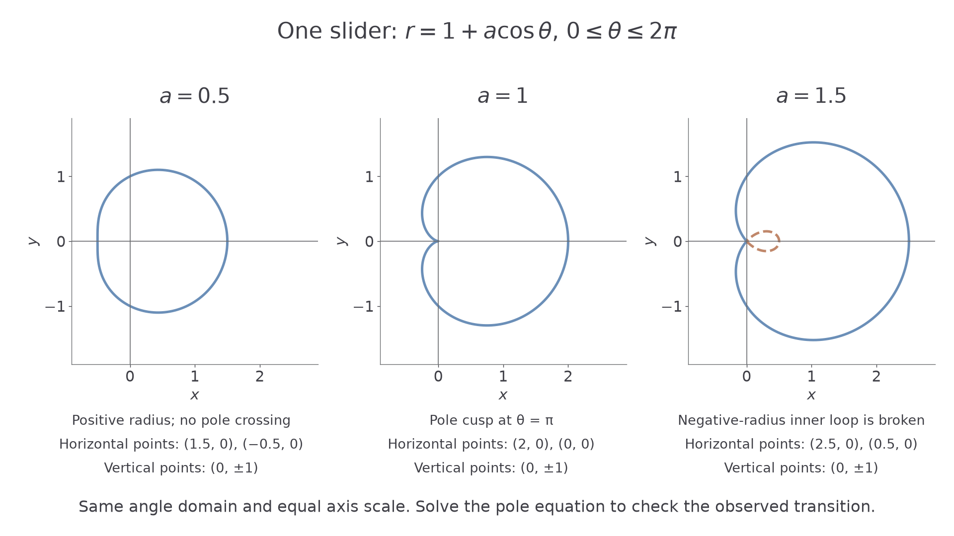
Plot $r=1+a\cos\theta$ with $0\le\theta\le2\pi$ and $0\le a\le2$ . Use equal axis scales, retain the full angle interval, and show negative- $r$ portions with broken lines. Increase the sampling density near the pole if a small loop is hard to see.

Replacing $\theta$ by $-\theta$ leaves $r$ unchanged, proving reflection symmetry in the initial line. Also $|r|\le1+a$ , so every fixed member is bounded. Being bounded does not mean that the same bound works for an unrestricted parameter family.

Pole and sign tests for this family

For $a\ge0$ ,

1-a\le r\le1+a

For $a>0$ , the pole condition is

\cos\theta=-1/a

Thus $a<1$ gives no pole point, $a=1$ gives a pole point at $\theta=\pi$ , and $a>1$ gives two pole angles with a negative- $r$ interval between them.

Not in the formula booklet: learn it.

These statements come from the cosine range and a solved equation. They describe the transition for every permitted parameter, rather than just the plotted snapshots.

Worked example 3: before the transition

Question. Describe the member $a=1/2$ , including its radial range, symmetry, pole behaviour and axis points.

Plan. Use the range first, then evaluate the coordinate-axis directions.

\begin{aligned} \frac12&\le r\le\frac32&&\text{cosine range}\\ r(0)&=\frac32,\quad r(\pi)=\frac12&&\text{horizontal directions}\\ r(\pi/2)&=r(3\pi/2)=1&&\text{vertical directions} \end{aligned}

Why this step? The strictly positive minimum proves that the curve never reaches the pole and has no negative- $r$ excursion.

Answer. A bounded closed curve, symmetric in the initial line, with axis points $(3/2,0)$ , $(-1/2,0)$ , $(0,\pm1)$ , and no pole crossing or inner loop.

Check. The horizontal point at $\theta=\pi$ lies left of the pole because its radius is positive.

Change only $a$ from $1/2$ to $3/2$ . The radial minimum becomes negative.

Worked example 4: after the transition

Question. Identify the inner-loop interval and key points when $a=3/2$ .

Plan. Solve the pole equation, check the sign between its roots, and convert the value at $\pi$ .

\begin{aligned} r=0&\Longleftrightarrow\cos\theta=-\frac23 &&\text{pole condition}\\ \alpha&=\arccos(-2/3),\quad \theta=\alpha,\ 2\pi-\alpha&&\text{two angles in the domain}\\ r<0&\Longleftrightarrow\alpha<\theta<2\pi-\alpha &&\text{negative cosine interval}\\ r(\pi)&=-\frac12 \Longrightarrow(x,y)=\left(\frac12,0\right) &&\text{reverse the direction} \end{aligned}

Why this step? The negative-radius section begins and ends at the pole; its plotted points form the inner loop on the right.

Answer. A bounded curve with an inner loop traced over $\alpha<\theta<2\pi-\alpha$ . Its outer horizontal tip is $(5/2,0)$ , its inner tip is $(1/2,0)$ , and its vertical-axis points are $(0,\pm1)$ . It remains symmetric in the initial line.

Check. Multiplying $r=-1/2$ by $\cos\pi=-1$ gives $x=1/2$ , fixing the loop's side.

At the transition $a=1$ , the plot has two branches meeting at the pole with a cusp. A later lesson verifies this kind of description by limiting tangent gradients. Here the pole equation identifies exactly where the visual transition occurs.

[DIAGRAM: asset_name: A polar slider crosses the loop transition; asset_slug: h645_b148_polar_family; caption: The same angle domain and axis scale reveal the change from a positive radius to a pole cusp and then an inner loop; description: Three equal-scale plots show r equals one plus a cosine theta for a equal to one half, one and three halves. The first has no pole crossing, the middle has a cusp at the pole and the last has a broken-line negative-radius inner loop on the right. Horizontal and vertical axis points are labelled in clear reserved positions.]
The same angle domain and axis scale reveal the change from a positive radius to a pole cusp and then an inner loop

Watch out

Wrong: infer “no loop” from a coarse plot or a cropped angle range. Right: solve $r=0$ , check signs, then refine the plot near the relevant parameter and angles.

Increase only the parameter once more.

Separate a tracing parameter from a family parameter

Now plot

x=t^2,\qquad y=t^3-at,\qquad t\in\mathbb R

Here $a$ chooses the curve and $t$ moves along it. A slider for $a$ must not replace the tracing parameter $t$ .

For an initial investigation, use $-1\le a\le4$ and $-3\le t\le3$ , then enlarge the $t$ -range to inspect the ends. The full curves are unbounded, although a finite parameter interval draws a bounded piece. Replacing $t$ by $-t$ preserves $x$ and reverses $y$ , proving symmetry in the horizontal axis.

Continue this lesson.

You’re previewing NovaLearn without an account. Create a free account to read the rest.

Create free account

Last Accessed

Core Pure

Mechanics (Major and Minor)

Statistics (Major and Minor)

Modelling with Algorithms

Numerical Methods

Extra Pure

Further Pure with Technology

TC1–TC5 - Families of curves with software

A slider suggests a pattern; algebra checks it

Use a polar slider to locate a loop transition

Separate a tracing parameter from a family parameter

Continue this lesson.

Learn faster with Nova