NU8 - Extrapolation from a sequence of estimates | OCR A-Level Further Mathematics B (MEI)

Use the pattern in a sequence of numerical estimates to improve its last value. Calculate and interpret ratios of differences, extrapolate to a finer calculation or to the limiting answer, cancel a leading step-length error, and justify the precision you report.

Find the pattern before extending it

A central difference calculation gives $1.0016675002$ for the gradient of $e^x$ at $x=0$ . A less accurate calculation gives $1.0066800127$ . Can the less accurate answer help improve the better one, without evaluating the function again?

It can, if you know how the errors change. The surprising part is that combining these two overestimates can give a slight underestimate. We will return to those numbers after learning how to recognise a useful error pattern.

You already know

Forward and central differences generally have method orders $1$ and $2$ . Midpoint and trapezium rules generally have order $2$ , and Simpson's rule generally has order $4$ . A method order describes error against step length; a sequence made by repeatedly reducing that step can still have first-order convergence. Retained spreadsheet values can be more precise than their displayed digits.

Extrapolation extends an observed pattern beyond the available calculations. Here the aim is usually to estimate the value approached as the numerical step tends to zero. It does not mean extending the integration interval beyond its endpoints.

Let $A_j$ be successive estimates of one fixed target $L$ . Use one subtraction direction throughout:

D_j=A_j-A_{j-1}

When one leading error term dominates and the refinement factor stays fixed, successive changes can approach a geometric pattern.

Ratio of successive differences

Provided $D_{j-1}\ne0$ , calculate

r_j=\frac{D_j}{D_{j-1}}

If these ratios appear to approach $r$ , with $|r|<1$ , a geometric model for the later changes may be useful. If the step is divided by $k>1$ each time and the method has leading error proportional to $h^p$ , the expected ratio is approximately

r=k^{-p}

Use the observed pattern to assess whether that model is appropriate.

Not in the formula booklet: learn it.

Do not infer a stable pattern from just one ratio. Check later rows, rounding effects and whether the same refinement factor was used. Negative ratios can describe alternating changes; they do not automatically mean divergence.

Worked example 1: decreasing trapezium estimates

Question. The trapezium rule gives the following output for a fixed integral. The number $n$ of equal strips doubles each row. Calculate the ratios of successive differences and suggest a useful limiting ratio.

$n$	$T_n$	Difference, new minus previous	Ratio
$4$	$1.727221904558$	—	—
$8$	$1.720518592164$	$-0.006703312393$	—
$16$	$1.718841128580$	$-0.001677463584$	$0.25024398$
$32$	$1.718421660316$	$-0.000419468264$	$0.25006103$
$64$	$1.718316786850$	$-0.000104873466$	$0.25001526$

Plan. Divide each new signed change by the preceding signed change, then link the trend to the halved width.

Using retained values,

\begin{aligned} r_{\mathrm{first}}&=\frac{-0.001677463584\ldots}{-0.006703312393\ldots} =0.25024398\ldots&&\text{same subtraction direction}\\ r_{\mathrm{next}}&=0.25006103\ldots&&\text{next refinement}\\ r_{\mathrm{last}}&=0.25001526\ldots&&\text{approaching }1/4\\ 1/4&=(1/2)^2&&\text{usual second-order behaviour} \end{aligned}

Why this step? Negative differences describe decreasing estimates. Dividing two successive negative differences gives a positive ratio, so the next change is predicted to have the same sign.

Answer. The ratios appear to converge to $r=1/4$ , consistent with a second-order method under halving.

Check. The changes get smaller in magnitude, and the ratios move closer to $1/4$ , rather than merely looking similar.

Change only the quadrature rule to midpoint, keeping the same integral and strip counts. The direction of the changes reverses, but the usual order does not.

Worked example 2: increasing midpoint estimates

Question. Interpret the corresponding midpoint output.

$n$	$M_n$	Difference, new minus previous	Ratio
$4$	$1.713815279771$	—	—
$8$	$1.717163664996$	$0.003348385225$	—
$16$	$1.718002192053$	$0.000838527057$	$0.25042730$
$32$	$1.718211913384$	$0.000209721331$	$0.25010681$
$64$	$1.718264349317$	$0.000052435933$	$0.25002670$

Plan. Keep the new-minus-previous convention and assess the same ratio trend.

\begin{aligned} r_{\mathrm{first}}&=\frac{0.000838527057\ldots}{0.003348385225\ldots} =0.25042730\ldots&&\text{successive positive changes}\\ r_{\mathrm{next}}&=0.25010681\ldots&&\text{later ratio}\\ r_{\mathrm{last}}&=0.25002670\ldots&&\text{closer to }1/4 \end{aligned}

Why this step? Using absolute differences throughout would hide whether the estimates rise, fall or alternate. Retaining signs prepares the correction in the next part.

Answer. A limiting ratio $r=1/4$ is again appropriate. The observed method order is $2$ , since the step is halved.

Check. The midpoint estimates increase while the trapezium estimates decrease towards the same region. Their common ratio pattern is compatible with that difference in direction.

Here the output agrees with the rules' usual orders. If the observed ratios instead settle near $0.36$ when $h$ is halved, use that evidence: the observed order is between $1$ and $2$ , because $1/4<0.36<1/2$ . Forcing $r=1/4$ would fit a different error model.

Exam tip

Identify a convergence trend, not just “approximately equal ratios”. Use retained values when available. A ratio formed from rounded display entries can differ from the spreadsheet's ratio without either calculation being mistyped.

Apply the same analysis to a fresh trapezium table.

Watch out

Wrong: decreasing estimates must give a negative successive-difference ratio. Their consistently defined differences are both negative, so their quotient is positive. Correct: here $r_j=D_j/D_{j-1}>0$ and approaches $1/4$ ; a negative ratio would describe alternating changes.

Keep the subtraction direction and the signs consistent in the next table.

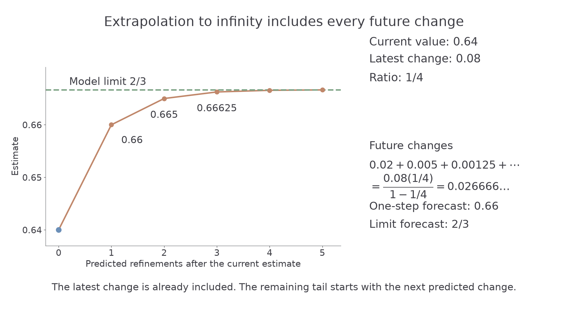
Add all the predicted future changes

Suppose the latest estimate is $A_j$ , its associated change is $D_j=A_j-A_{j-1}$ , and the later change ratio is modelled by $r$ . The next change is predicted to be $rD_j$ . The change $D_j$ has already been included in $A_j$ .

A one-step forecast is therefore $A_{j+1}\approx A_j+rD_j$ . To estimate the limit, add the whole remaining geometric tail:

L\approx A_j+D_j(r+r^2+r^3+\cdots)

For $|r|<1$ , that tail sums to $D_jr/(1-r)$ . The infinite geometric-series sum is in the formula booklet; its application to the remaining error gives the extrapolation formula below.

Extrapolation to the limit

For a useful geometric model of later signed changes, with $|r|<1$ ,

E=A_j+\frac{rD_j}{1-r}, \qquad D_j=A_j-A_{j-1}

Equivalently, starting at the previous estimate,

E=A_{j-1}+\frac{D_j}{1-r}

These are the same calculation. A single predicted refinement $A_j+rD_j$ is only partial extrapolation.

Not in the formula booklet: learn it.

The formula follows from summing predicted future changes. It is exact for an exact geometric error model and approximate when the ratios only tend towards a limit.

[DIAGRAM: asset_name: The remaining geometric tail contains more than the next step; asset_slug: h645_b133_geometric_tail; caption: With current value 0.64, latest change 0.08 and ratio one quarter, the next change is 0.02 but all future changes sum to 0.026666 recurring; description: A plot shows a geometric model beginning at the current estimate 0.64 and predicting 0.66, 0.665, 0.66625 and further values towards two thirds. A sage horizontal line marks the model limit. Blue marks the current estimate and clay marks predicted refinements. A separate notes panel lists future changes 0.02, 0.005, 0.00125 and so on, then their sum 0.026666 recurring. It contrasts the one-step forecast 0.66 with the limiting forecast two thirds.]
With current value 0.64, latest change 0.08 and ratio one quarter, the next change is 0.02 but all future changes sum to 0.026666 recurring

The following table illustrates why an observed ratio can matter more than a rule's usual theoretical order. The integrand is $\sqrt{x}$ on $[0,1]$ , whose gradient is unbounded near $0$ .

Worked example 3: an increasing sequence with an unusual ratio

Question. Use the trapezium output to extrapolate to the limiting integral. Use the last observed ratio, and give a reasonable improved estimate to $5$ decimal places.

$n$	$T_n$	Difference	Ratio
$4$	$0.643283046243$	—	—
$8$	$0.658130221624$	$0.014847175382$	—
$16$	$0.663581196877$	$0.005450975253$	$0.36713887$
$32$	$0.665558936279$	$0.001977739402$	$0.36282304$
$64$	$0.666270811379$	$0.000711875100$	$0.35994383$
$128$	$0.666525657297$	$0.000254845918$	$0.35799246$

Plan. Use the latest estimate, its own signed difference and the observed ratio to add the entire predicted tail.

\begin{aligned} A_j&=0.666525657297\ldots&&\text{latest estimate}\\ D_j&=0.000254845918\ldots,\quad r\approx0.35799246 &&\text{matching change and ratio}\\ E&=0.666525657297\ldots+ 0.000254845918\ldots\frac{0.35799246}{1-0.35799246} &&\text{all future changes}\\ &\approx0.666667762976&&\text{retain working digits} \end{aligned}

Why this step? The ratios are moving towards about $0.35$ , not $0.25$ . The usual second-order trapezium model is not the observed behaviour for this endpoint-sensitive integrand.

Answer. A reasonable improved estimate is $0.66667$ to $5$ decimal places. The settling ratios support geometric-tail correction, which removes much of the remaining error in the raw value. This is an accuracy judgement based on the model, rather than a guaranteed error bound.

Check. The correction is positive, continuing the rising sequence. For this example, direct integration gives $2/3=0.666666\ldots$ ; the extrapolated estimate has absolute error about $0.0000010963$ , much smaller than the raw estimate's error of about $0.0001410094$ .

Continue this lesson.

You’re previewing NovaLearn without an account. Create a free account to read the rest.

Create free account

Last Accessed

Core Pure

Mechanics (Major and Minor)

Statistics (Major and Minor)

Modelling with Algorithms

Numerical Methods

Extra Pure

Further Pure with Technology

NU8 - Extrapolation from a sequence of estimates

Find the pattern before extending it

Add all the predicted future changes

Continue this lesson.

Learn faster with Nova