AA4–AA6 - Efficiency, correctness and heuristics | OCR A-Level Further Mathematics B (MEI)

An algorithm needs more than a correct-looking answer on one input. You will count its work, compare how that work grows, distinguish a proof from a collection of tests, and explain why a useful heuristic need not guarantee an optimal solution.

Count the specified operation before giving an order

Can an algorithm pass a hundred tests and still be wrong? Yes: testing gives evidence about the cases tested. Before deciding what has been established, separate three questions: does the procedure work, how much work does it need, and does it find the best answer?

You already know

Algorithms use initial states, sequential updates, conditions and stopping rules. Trace the given instructions faithfully. A finite sequence of successful examples does not by itself prove a claim about every integer.

To compare efficiency, state what measures the problem size and what operation is being counted. For sorting, the size might be the number of items and the operation a comparison. For a nested loop, it might be an execution of the loop's main instruction.

Complexity and worst case

Algorithmic complexity describes how a measure of the work grows with the problem size $n$ . Worst-case complexity considers inputs of size $n$ requiring the greatest amount of that work.

Order notation such as $O(n^2)$ describes a growth bound for large $n$ . In ordinary polynomial-order comparisons, report the dominant growth: constant factors and lower-power terms do not change that classification.

For example, $3n^2+7n+2$ has quadratic order $O(n^2)$ . That does not mean it performs exactly $n^2$ operations, or that every quadratic algorithm is faster than every cubic algorithm for a small input. Constants and implementation details still affect actual timings.

Worked example 1: a triangular nested loop

Question. A counter $C$ starts at zero. For each $i=1,\ldots,n$ , an inner loop runs for $j=1,\ldots,i$ , increasing $C$ by one each time. The procedure outputs $C$ . Count these counter increases when $n=5$ , and give the order for general $n$ . Do not count loop-control tests.

Plan. Count the inner-loop executions for each value of $i$ , then sum.

\begin{aligned} C(5)&=1+2+3+4+5=15\\ C(n)&=1+2+\cdots+n=\frac{n(n+1)}{2}\\ &=\frac12n^2+\frac12n\\ \text{order}&=O(n^2) \end{aligned}

Why this step? The inner loop has a different length for each $i$ . Multiplying $n$ by the first inner-loop length would miss most of the work.

Answer. $15$ counter increases for $n=5$ ; quadratic order $O(n^2)$ .

Check. The exact count lies below $n^2=25$ , but its leading term is still proportional to $n^2$ .

Change only the inner-loop upper bound, from $i$ to $n$ . The order may stay the same even though the exact count changes.

Worked example 2: a rectangular nested loop

Question. Now the inner loop runs for $j=1,\ldots,n$ for every $i=1,\ldots,n$ . Count counter increases for $n=5$ , and give the general order.

Plan. Multiply the number of outer iterations by the fixed number of inner iterations.

\begin{aligned} C(5)&=5(5)=25\\ C(n)&=\underbrace{n+\cdots+n}_{n\text{ terms}}=n^2\\ \text{order}&=O(n^2) \end{aligned}

Why this step? Both loop ranges grow with the input, so their work multiplies rather than adds.

Answer. $25$ counter increases for $n=5$ ; order $O(n^2)$ .

Check. The rectangular loop performs more increases than the triangular loop, but both have quadratic dominant growth.

The arithmetic-series formula is supplied in the formula booklet; these algorithm-specific counts and complexity interpretations are not.

Watch out

Wrong: call two successive loops quadratic merely because there are two loops.

Right: successive loop counts add; nested loop counts may multiply. Count the specified operation using the actual ranges.

Change the triangular loop's inner range once more.

Scale the problem and count repeated runs

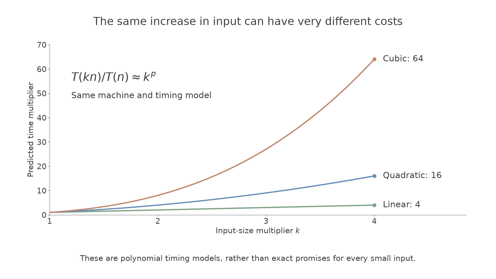
For large problems on the same machine, an operation count often supplies a useful timing model. State the model: an order classification alone is not a promise of an exact number of seconds.

Polynomial timing model

If the running time is modelled by $T(n)\approx cn^p$ , with the same constant $c$ , multiplying the size by $k$ multiplies the predicted time by $k^p$ :

\frac{T(kn)}{T(n)}\approx k^p

If that procedure is run $n$ times on size- $n$ inputs, its total modelled time is proportional to $n^{p+1}$ .

Not in the formula booklet: learn it.

Use the size variable specified in the question. Doubling the number of vertices and doubling the number of edges are not interchangeable descriptions of a network problem.

[DIAGRAM: asset_name: Input and timing multipliers; asset_slug: h645_b110_polynomial_scaling; caption: The growth power applies to the input-size multiplier; description: Exact graphs on input-size multiplier k from one to four show linear time multiplier k in sage, quadratic multiplier k squared in blue and cubic multiplier k cubed in clay. At input multiplier four, the time multipliers are four, sixteen and sixty-four. The axes are labelled input-size multiplier and predicted time multiplier.]
The growth power applies to the input-size multiplier

Worked example 3: scaling one quadratic run

Question. A procedure has a quadratic timing model. One run on a problem of size $50$ takes $0.2$ seconds. Estimate the time for one run on size $150$ , on the same machine.

Plan. Find the size multiplier and square it.

\begin{aligned} k&=\frac{150}{50}=3\\ T(150)&\approx0.2(3^2)\\ &=1.8\,\mathrm s \end{aligned}

Why this step? A quadratic model squares the size multiplier; multiplying the time merely by three would use a linear model.

Answer. Approximately $1.8$ seconds.

Check. The size is three times as large and the predicted time nine times as large.

Change only the task: instead of one run, apply the size- $n$ procedure once for each of $n$ starting positions.

Worked example 4: quadratic work repeated n times

Question. Using the same timing model, estimate the total time at size $150$ when the procedure is run $150$ times. State the total order as a function of $n$ .

Plan. First use the time for one run, then multiply by the number of runs.

\begin{aligned} T_{\mathrm{total}}(150)&\approx150(1.8)=270\,\mathrm s\\ T_{\mathrm{total}}(n)&\approx n(cn^2)=cn^3\\ \text{total order}&=O(n^3) \end{aligned}

Why this step? The number of repetitions grows with the problem size. It is not a fixed constant that can be ignored in the order.

Answer. Approximately $270$ seconds, with cubic total order $O(n^3)$ .

Check. At size $50$ , the repeated task takes $50(0.2)=10$ seconds. Increasing the size by three multiplies this total by $3^3=27$ , giving $270$ .

Continue this lesson.

You’re previewing NovaLearn without an account. Create a free account to read the rest.

Create free account

Last Accessed

Core Pure

Mechanics (Major and Minor)

Statistics (Major and Minor)

Modelling with Algorithms

Numerical Methods

Extra Pure

Further Pure with Technology

AA4–AA6 - Efficiency, correctness and heuristics

Count the specified operation before giving an order

Scale the problem and count repeated runs

Continue this lesson.

Learn faster with Nova