8.05e–8.05g - Stationary points and tangent planes | OCR A-Level Further Mathematics A

Find the stationary points of a surface and classify them using the Hessian matrix. You will handle coupled equations and an inconclusive determinant, then find tangent planes from the height and the two coordinate gradients.

Finding stationary points

If a surface has a horizontal tangent plane, must the point be a top or a bottom? At the origin, both $z=x^2+y^2$ and $z=x^2-y^2$ have zero gradients in the coordinate directions. Yet one is a bowl and the other is a saddle. Zero slopes identify a candidate; the behaviour nearby decides its nature.

You already know

For $z=f(x,y)$ , $f_x$ holds $y$ fixed and $f_y$ holds $x$ fixed. Calculate $f_{xx},f_{xy},f_{yx},f_{yy}$ by differentiating again. A plane $ax+by+cz=d$ has normal vector $(a,b,c)$ .

At a differentiable stationary point, both coordinate gradients vanish. Solving the two equations gives horizontal coordinates, but a point on a surface needs a height as well.

Stationary point

A stationary point of $z=f(x,y)$ occurs where $f_x=f_y=0$ . Its coordinates are $(a,b,f(a,b))$ , where $(a,b)$ solves both equations simultaneously.

The condition $f_x=f_y=0$ is not printed as a separate result in the formula booklet. The booklet's Hessian test assumes that you have already found a stationary point. These equations concern differentiable interior points; they do not locate every possible extremum on a restricted boundary.

Worked example 1: two stationary points

Question. Find the stationary points of $z=x^3+y^2-3x$ .

Plan. Set both first partial derivatives to zero, solve simultaneously, and calculate the heights.

\begin{aligned} f_x&=3x^2-3,& f_y&=2y && \text{differentiate}\\ 3x^2-3&=0,& 2y&=0 && \text{stationary conditions}\\ x&=\pm1,& y&=0 && \text{solve both equations}\\ f(1,0)&=1-3=-2 && \text{first height}\\ f(-1,0)&=-1+3=2 && \text{second height} \end{aligned}

Why this step? $(1,0)$ and $(-1,0)$ are positions in the horizontal plane; the question asks for points on the three-dimensional surface.

Answer. $(1,0,-2)$ and $(-1,0,2)$ .

Check. At either position, $3x^2-3=0$ and $2y=0$ , so both first partial derivatives vanish.

Worked example 2 changes only the coefficient of $x$ . Keep the same sequence, including the height calculation.

Worked example 2: a changed coefficient

Question. Find the stationary points of $z=x^3+y^2-12x$ .

Plan. Solve $f_x=f_y=0$ and substitute each solution into the original surface.

\begin{aligned} f_x&=3x^2-12,& f_y&=2y && \text{first derivatives}\\ x^2&=4,& y&=0 && \text{set both to zero}\\ x&=2\text{ or }-2 && \text{both roots}\\ f(2,0)&=8-24=-16 && \text{height at }x=2\\ f(-2,0)&=-8+24=16 && \text{height at }x=-2 \end{aligned}

Why this step? The two signs give distinct stationary points, and neither is removed by the other equation.

Answer. $(2,0,-16)$ and $(-2,0,16)$ .

Check. At $x=\pm2$ , $f_x=3(4)-12=0$ ; at $y=0$ , $f_y=0$ .

Finding the points does not yet establish whether they are maxima, minima or saddles.

Watch out

Wrong: report only $(2,0)$ and $(-2,0)$ as stationary points of a surface. Right: substitute back for $z$ and report all three coordinates. Also solve both derivative equations: $f_x=0$ alone describes possible positions, not necessarily stationary points.

The next check changes the linear coefficient again.

Classifying with the Hessian

A local minimum lies below or at all sufficiently nearby points of the surface; a local maximum lies above or at them. At a saddle-point there are points both above and below its height arbitrarily close to it.

The coordinate sections alone can mislead you. For $z=x^2+4xy+y^2$ , both sections $x=0$ and $y=0$ curve upwards at the origin. But along $y=-x$ ,

z=x^2-4x^2+x^2=-2x^2<0\quad(x\ne0),

while along $y=0$ , $z=x^2>0$ . The origin is a saddle. You need a test that includes the mixed term.

Hessian matrix

For a surface with continuous second partial derivatives near the point, the Hessian matrix is

\mathbf H= \begin{pmatrix} f_{xx}&f_{xy}\\ f_{yx}&f_{yy} \end{pmatrix}.

Its determinant is $D=\det\mathbf H=f_{xx}f_{yy}-(f_{xy})^2$ , using $f_{xy}=f_{yx}$ . The matrix is not its determinant: $\mathbf H$ has four entries, while $D$ is a number.

Evaluate the entries at the stationary point before applying the test. A Hessian evaluated somewhere else describes a different position.

Hessian test at a stationary point

For a stationary point of $z=f(x,y)$ , with continuous second partial derivatives nearby, let $D=\det\mathbf H$ at that point.

Conditions	Nature
$D>0$ and $f_{xx}>0$	local minimum
$D>0$ and $f_{xx}<0$	local maximum
$D<0$	saddle-point
$D=0$	test is inconclusive

In the formula booklet.

Why does the mixed term matter? Near a stationary point, the curvatures combine in the expression $f_{xx}u^2+2f_{xy}uv+f_{yy}v^2$ . For $f_{xx}\ne0$ , completing the square gives

f_{xx}\left(u+\frac{f_{xy}}{f_{xx}}v\right)^2+\frac{D}{f_{xx}}v^2.

When $D>0$ , both coefficients have the sign of $f_{xx}$ . When $D<0$ , the expression takes both signs. This explains the booklet's test; it is not a separate formula to memorise. If $f_{xx}=0$ but $D<0$ , the mixed term still produces both signs. No conclusion follows from $D=0$ alone.

Worked example 3: a minimum

Question. Classify the stationary point at the origin of $z=x^2+xy+y^2$ .

Plan. Find the Hessian entries, calculate its determinant and use its sign with $f_{xx}$ .

\begin{aligned} f_{xx}&=2,& f_{xy}=f_{yx}&=1,& f_{yy}&=2 && \text{second derivatives}\\ \mathbf H&=\begin{pmatrix}2&1\\1&2\end{pmatrix} && \text{Hessian at the origin}\\ D&=2(2)-1^2=3>0 && \text{determinant}\\ f_{xx}&=2>0 && \text{upward curvature} \end{aligned}

Why this step? A positive determinant separates extrema from saddles, but its sign alone does not distinguish a maximum from a minimum.

Answer. The origin is a local minimum.

Check. $x^2+xy+y^2=(x+y/2)^2+3y^2/4$ , which is positive away from the origin and zero there.

Worked example 4 changes only the overall sign of the surface. The determinant stays positive, but the curvatures reverse.

Worked example 4: a maximum

Question. Classify the stationary point at the origin of $z=-x^2-xy-y^2$ .

Plan. Recalculate the signed entries and distinguish the extremum using $f_{xx}$ .

\begin{aligned} \mathbf H&=\begin{pmatrix}-2&-1\\-1&-2\end{pmatrix} && \text{second derivatives}\\ D&=(-2)(-2)-(-1)^2=3>0 && \text{determinant}\\ f_{xx}&=-2<0 && \text{downward curvature} \end{aligned}

Why this step? Negating every entry multiplies a determinant of order two by $(-1)^2=1$ , so $D$ cannot distinguish these two surfaces on its own.

Answer. The origin is a local maximum.

Check. $z=-(x+y/2)^2-3y^2/4\le0$ , with equality only at the origin.

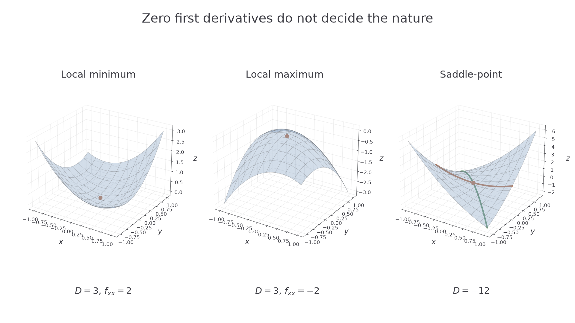
A picture makes the three possible conclusive outcomes distinct.

[DIAGRAM: asset_name: A minimum, a maximum and a saddle; asset_slug: h245_8_05_stationary_types; caption: A stationary point can be a local minimum, a local maximum or a saddle.; description: Three exact three-dimensional plots near the origin: z=x squared+xy+y squared with D=3 and fxx=2; z=-x squared-xy-y squared with D=3 and fxx=-2; z=x squared+4xy+y squared with D=-12. All show the origin. The saddle highlights the upward section y=0 and the downward section y=-x.]
A stationary point can be a local minimum, a local maximum or a saddle.

Watch out

Wrong: $D>0$ means a minimum. Right: also inspect $f_{xx}$ : positive gives a minimum, negative gives a maximum. When $D<0$ , the point is a saddle regardless of the sign of $f_{xx}$ .

For the next surface, the stationary point is already given, so focus on the classification.

Coupled stationary equations

When each first derivative contains both variables, solve the stationary equations simultaneously without discarding zero solutions.

For $z=x^3+y^3-6xy$ , the equations are $x^2=2y$ and $y^2=2x$ . Dividing one equation by $x$ at the start would lose the origin. Substitute one expression into the other and factor instead.

Worked example 5: preserving the zero solution

Question. Determine and classify all stationary points of $z=x^3+y^3-6xy$ .

Plan. Eliminate $y$ by substitution, retain every factor, then evaluate the height and Hessian at each solution.

\begin{aligned} f_x=0&\ \Rightarrow\ x^2=2y,& f_y=0&\ \Rightarrow\ y^2=2x && \text{first derivatives divided by }3\\ y&=\frac{x^2}{2},& \frac{x^4}{4}&=2x && \text{substitute}\\ x(x^3-8)&=0 && \text{retain the zero factor}\\ (x,y)&=(0,0)\text{ or }(2,2) && \text{real solutions}\\ f(0,0)&=0,& f(2,2)&=8+8-24=-8 && \text{heights} \end{aligned}

The second derivatives give

\begin{aligned} \mathbf H&=\begin{pmatrix}6x&-6\\-6&6y\end{pmatrix} & D&=36xy-36 && \text{determinant as a function}\\ D(0,0)&=-36<0 && \text{saddle test}\\ D(2,2)&=108>0,& f_{xx}(2,2)&=12>0 && \text{minimum test} \end{aligned}

Why this step? Factoring $x(x^3-8)$ , rather than dividing by $x$ , preserves the stationary point that would otherwise disappear.

Answer. A saddle-point at $(0,0,0)$ and a local minimum at $(2,2,-8)$ .

Check. Both pairs satisfy $x^2=2y$ and $y^2=2x$ . A real cubic equation $x^3=8$ has just the real solution $x=2$ , so no real solutions were omitted.

Continue this lesson.

You’re previewing NovaLearn without an account. Create a free account to read the rest.

Create free account

Last Accessed

Pure Core

Statistics

Mechanics

Discrete Mathematics

Additional Pure Mathematics

8.05e–8.05g - Stationary points and tangent planes

Finding stationary points

Classifying with the Hessian

Coupled stationary equations

Continue this lesson.

Learn faster with Nova