7.06d - Solving linear programmes graphically | OCR A-Level Further Mathematics A

Use a graph to find and interpret the optimum of a linear programme in two variables. You will leave the feasible region unshaded, compare its vertices, handle whole-number solutions and recognise when a problem has several optima or no optimum.

Drawing the feasible region

Can rounding a correct graphical optimum give a feasible answer that still loses money? It can. First we need a graph that shows exactly which choices are permitted; later we will see why the nearest lattice point need not be the best one.

You already know

A linear programme has a linear objective, linear constraints and restrictions such as $x, y \ge 0$ . The line $ax + by = c$ is the boundary of $ax + by \le c$ ; a test point tells you which side satisfies the inequality.

Draw each boundary accurately using two points. For $x + 2y = 8$ , the intercepts are $(8, 0)$ and $(0, 4)$ . A boundary is solid when equality is included. Test a point that is not on the boundary; the origin is convenient when it is available, but it cannot distinguish the sides of a line through the origin.

Feasible region

The feasible region consists of all points satisfying every constraint. Its boundary is included wherever the corresponding inequality allows equality. For an integer problem, only the lattice points in this region are permitted solutions.

Use OCR's shading convention: shade the side that does not satisfy each inequality. The points surviving every exclusion form the unshaded feasible region. Label it so that overlapping shading cannot obscure its meaning.

Worked example 1: excluding the wrong side

Question. Represent $x + 2y \le 8$ graphically in the first quadrant.

Plan. Draw the boundary, test the origin and shade the excluded side.

\begin{aligned} y = 0 &\Rightarrow x = 8 && \text{horizontal intercept} \\ x = 0 &\Rightarrow y = 4 && \text{vertical intercept} \\ (0, 0):\quad 0 + 2(0) &= 0 \le 8 && \text{origin satisfies the constraint} \end{aligned}

Why this step? A straight boundary divides the plane into two half-planes, and the inequality has the same truth value throughout either open half-plane.

Answer. Draw a solid line through $(8, 0)$ and $(0, 4)$ . Leave its origin side unshaded and shade above the line; also exclude negative $x$ and negative $y$ .

Check. $(2, 2)$ remains, since $2 + 4 = 6 \le 8$ ; $(4, 3)$ is excluded, since $4 + 6 = 10 > 8$ .

The next example changes only the inequality sign. The boundary stays exactly where it was; the permitted side changes.

Worked example 2: reversing the permitted side

Question. Represent $x + 2y \ge 8$ graphically in the first quadrant.

Plan. Use the same boundary but repeat the test-point decision.

\begin{aligned} x + 2y &= 8 && \text{same solid boundary} \\ (0, 0):\quad 0 &\not\ge 8 && \text{origin is now excluded} \end{aligned}

Why this step? The sign, rather than the appearance of the line, decides which side is allowed.

Answer. Shade the side containing the origin and leave the side above the line unshaded, within the first quadrant.

Check. The earlier test points exchange roles: $(2, 2)$ fails, while $(4, 3)$ satisfies the new inequality.

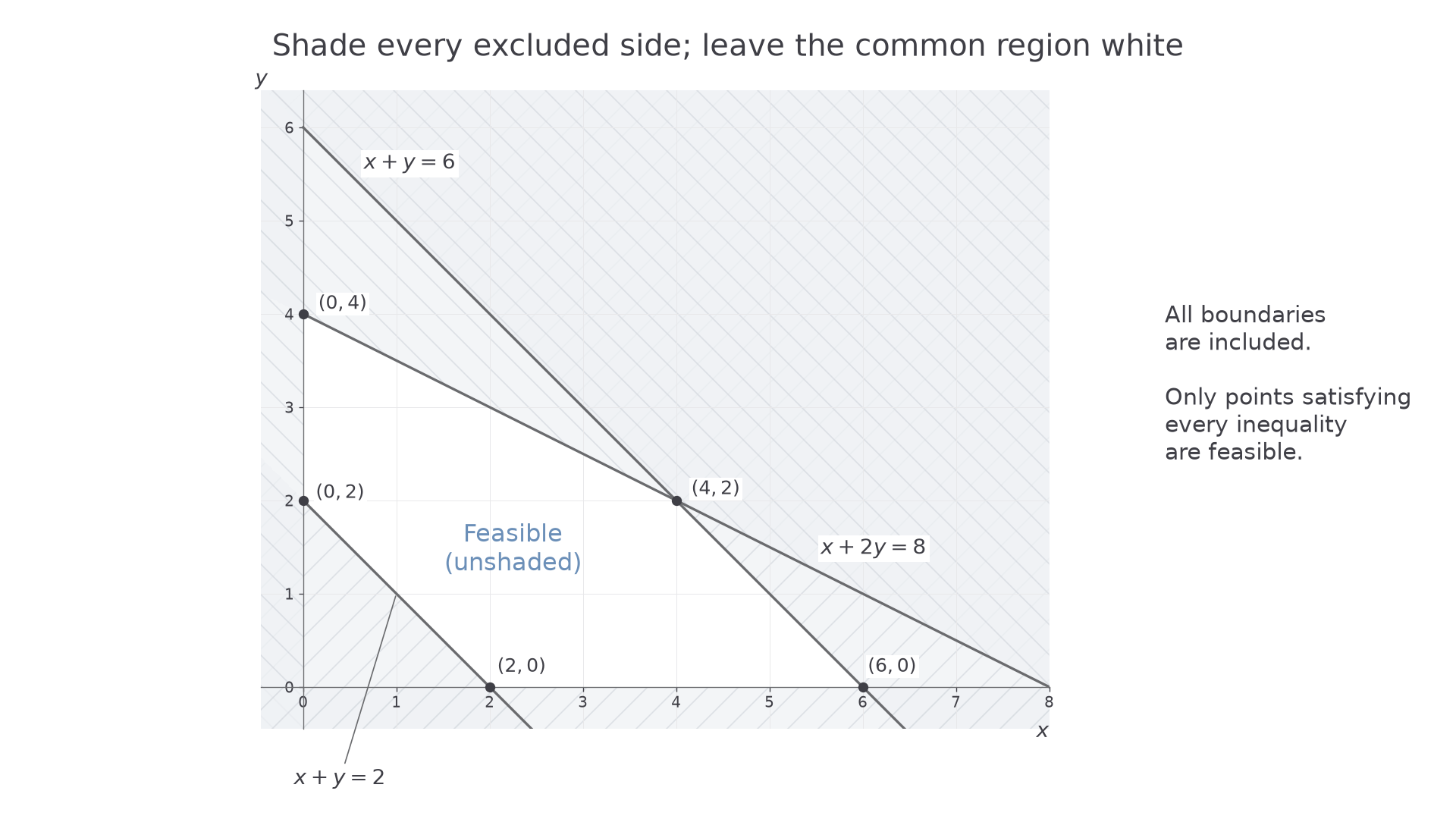
For several inequalities, repeat this process on the same axes. The following region satisfies $x + y \le 6$ , $x + 2y \le 8$ , $x + y \ge 2$ and $x, y \ge 0$ . Its five vertices are where the surviving boundary segments meet.

[DIAGRAM: asset_name: Excluded half-planes leave a feasible polygon; asset_slug: h245_7_06_feasible_region; caption: The unshaded polygon satisfies all five constraints, including the minimum total x + y = 2; description: Equal-scale first-quadrant axes show solid boundaries x + y = 6, x + 2y = 8 and x + y = 2. Excluded half-planes are pale and hatched; the central feasible pentagon is white and labelled feasible. Its vertices are labelled (0,2), (2,0), (6,0), (4,2), (0,4). Labels distinguish each line without overlap]
The unshaded polygon satisfies all five constraints, including the minimum total x + y = 2

Watch out

Wrong: shade the side satisfying each constraint. OCR asks for the reverse convention: shade each excluded side, leaving the feasible region unshaded. The inequalities still decide the answer even if several shaded regions overlap.

Use a point off the boundary to make the next decision.

Vertices and objective lines

The objective selects the best point inside the feasible region; it does not supply another constraint.

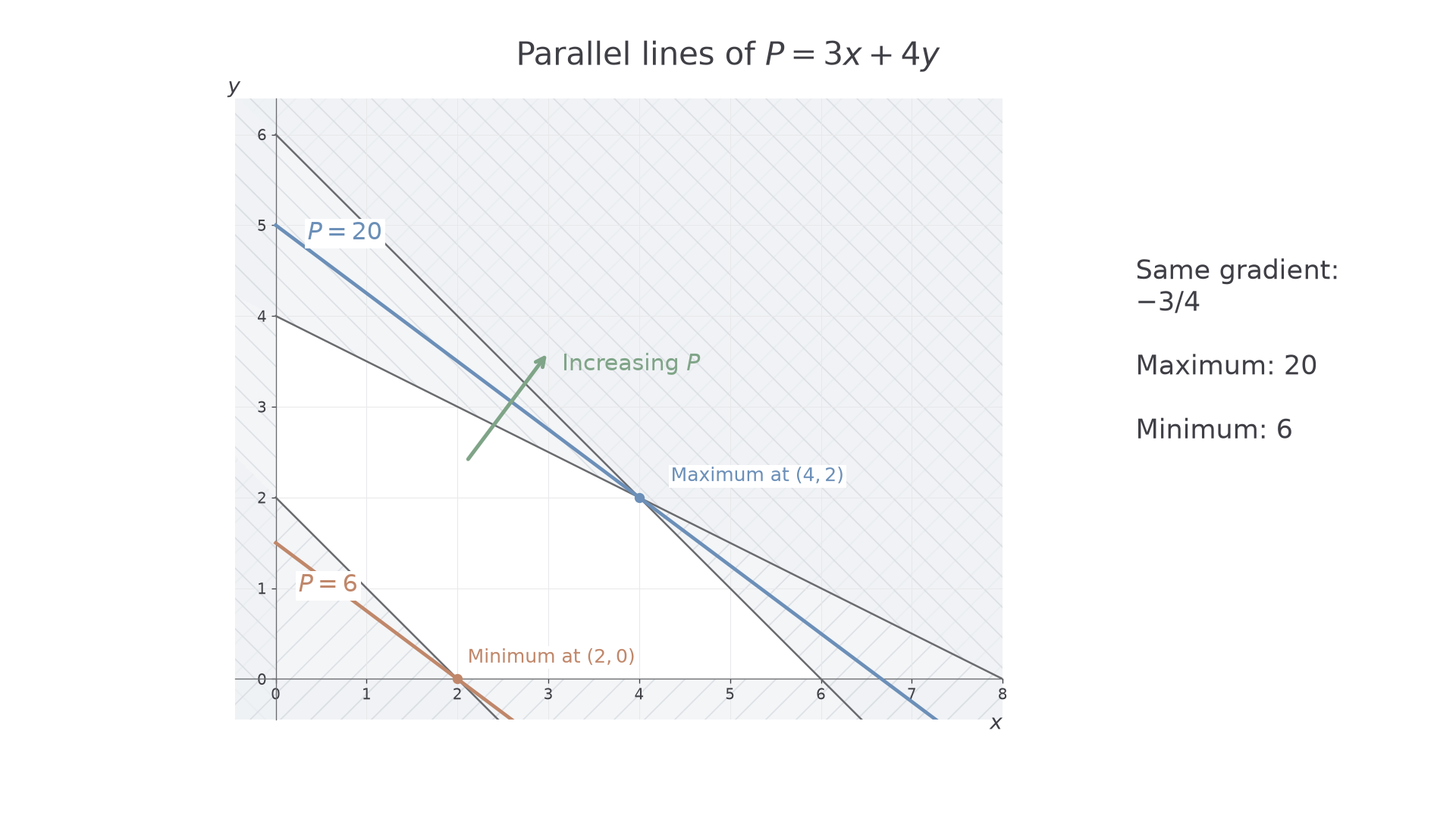
For $P = 3x + 4y$ , the equations $3x + 4y = k$ form parallel lines of gradient $-3/4$ . Increasing $k$ moves the line towards greater objective values. Slide a ruler parallel to this line until its final contact with the feasible region to locate a maximum; move towards smaller $k$ for a minimum.

For a non-empty bounded polygon, a linear objective has an optimum at a vertex. Here is why. Every point on an edge is a weighted average of its endpoints, so its objective is the same weighted average of their objective values: it cannot exceed both endpoints. Interior points are weighted averages of vertices, with the same conclusion. An entire edge may tie for the optimum, but at least one vertex always attains it. These graphical results are not in the formula booklet: learn them.

Worked example 3: maximising at a vertex

Question. Maximise $P = 3x + 4y$ , subject to $x + y \le 6$ , $x + 2y \le 8$ , $x + y \ge 2$ and $x, y \ge 0$ .

Plan. Draw the feasible region, find its vertices exactly and compare the objective values.

The two upper sloping boundaries meet where

\begin{aligned} x + y &= 6 && \text{first boundary} \\ x + 2y &= 8 && \text{second boundary} \\ y &= 2,\quad x = 4 && \text{subtract and substitute} \end{aligned}

The remaining vertices are the axis intersections surviving all constraints.

Vertex	$3x + 4y$
$(0, 2)$	$8$
$(2, 0)$	$6$
$(6, 0)$	$18$
$(4, 2)$	$20$
$(0, 4)$	$16$

Why this step? A vertex comparison proves the best value over the whole polygon, not just over a few chosen feasible points.

Answer. The maximum is $P = 20$ , at $(x, y) = (4, 2)$ .

Check. At this point, the upper constraints give $6$ and $8$ , and the lower total is $6 \ge 2$ . A larger parallel objective line misses the region.

The next example changes only “maximise” to “minimise”. No boundary or objective gradient changes.

Worked example 4: minimising the same objective

Question. Minimise $P = 3x + 4y$ over the same feasible region.

Plan. Use the existing vertex values and select the smallest, interpreting the opposite direction of travel of the objective line.

\begin{aligned} P_{\min} &= \min\{8, 6, 18, 20, 16\} && \text{compare all vertices} \\ &= 6 && \text{at } (2, 0) \end{aligned}

Why this step? The origin would have objective zero, but it violates $x + y \ge 2$ , so it cannot be considered.

Answer. The minimum is $P = 6$ , at $(x, y) = (2, 0)$ .

Check. The point satisfies $2 \le 6$ , $2 \le 8$ and $2 \ge 2$ ; a smaller objective line has no feasible point.

The parallel lines in the picture record both directions of optimisation.

[DIAGRAM: asset_name: Parallel objective lines locate both optima; asset_slug: h245_7_06_objective_lines; caption: The line 3x + 4y = 20 meets the feasible region last at (4,2) when maximising; the line 3x + 4y = 6 meets it first at (2,0) when minimising; description: Equal-scale axes show the same white feasible pentagon with excluded regions shaded. A blue objective line through (4,2) is labelled P = 20, and a parallel clay objective line through (2,0) is labelled P = 6. A clear arrow normal to the lines points towards increasing P. Both optimal points have separate readable labels]
The line 3x + 4y = 20 meets the feasible region last at (4,2) when maximising

Exam tip

Read a promising optimum from the graph, then solve the active boundary equations to obtain exact coordinates. Finish with the objective value and what the variables represent when the problem has a context.

The next objective has a different gradient, so do not assume the previous optimum survives.

Continue this lesson.

You’re previewing NovaLearn without an account. Create a free account to read the rest.

Create free account

Last Accessed

Pure Core

Statistics

Mechanics

Discrete Mathematics

Additional Pure Mathematics

7.06d - Solving linear programmes graphically

Drawing the feasible region

Vertices and objective lines

Continue this lesson.

Learn faster with Nova