5.02i–5.02l - The Poisson distribution as a model
Recognise a Poisson count, scale its parameter to the stated interval, calculate exact and cumulative probabilities, and explain its modelling assumptions in context. The model describes random event counts over time, distance or area.
Random counts in a fixed interval
A help desk receives calls at an average of per minutes. Does “average” mean exactly three calls every ten minutes, or one call regularly every seconds? Neither: the Poisson model allows empty intervals and busy ones. How can a steady average coexist with such uneven counts?
You already know
A discrete distribution assigns probabilities to integer outcomes. Distinguish an average rate from a particular observed count, and convert units before calculating with a rate.
Split a time interval into many tiny pieces. If events happen independently at a constant average rate, most pieces contain no event, a few contain one, and a piece containing several becomes negligible as its length shrinks. Counting events across the whole interval leads to the Poisson pattern. This is an informal model explanation, not a request for a limiting calculation or an approximation to a binomial probability.
Poisson distribution as a count model
Write when is modelled as the number of separate events in a specified interval with Poisson parameter , the average number for that interval. Its possible values are , with no fixed upper limit. The modelling assumptions to assess are independently occurring events and a constant average rate over the interval.
An interval can be a length, area or volume as well as time. Under a constant average rate per unit, an interval of size has parameter . This rate-to-interval relationship and the modelling conditions are not in the formula booklet: learn them. The parameter must describe the whole region or interval being counted, not one unit unless one unit is actually requested.
For the desk, minutes has parameter , whereas minutes has parameter . A parameter need not be an integer even though every realised count is an integer.
[DIAGRAM: asset_name: Random events and a constant average rate; asset_slug: h245_5_02_poisson_intervals; caption: At 3 calls per 10 minutes, the Poisson parameter for 20 minutes is 6. A possible sequence of calls is irregular; the two ten-minute counts need not both be 3; description: A twenty-minute timeline shows seven possible event times with four in the first half and three in the second. Brackets mark two ten-minute intervals and the whole twenty-minute interval. Text distinguishes the observed count 7 from the model parameter 6 and says the average rate does not prescribe regular spacing]
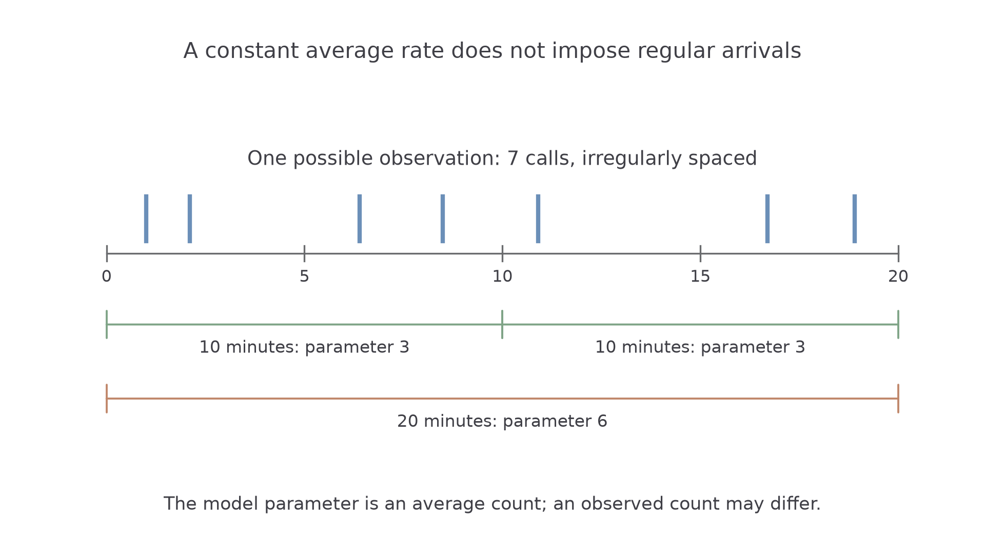
The diagram's seven calls are one possible observation, not an error in a model with parameter .
Key idea
Poisson randomness concerns the event count; a constant average rate does not mean equal gaps between events.
Identify both what is counted and the size of its interval.
Calculating an exact count probability
The Poisson formula turns the interval parameter into the probability of a particular count. It includes zero events, which is often a useful probability in its own right.
Poisson probability mass
For , with , and ,
Recall that , so .
In the formula booklet.
For adjacent masses, dividing the formulae gives . This ratio is not separately in the booklet. It explains why probabilities first rise and then fall when , rather than always decreasing as in a geometric model.
Worked example 1: scale the interval first
Question. Calls arrive under Poisson conditions at an average of per minutes. Find the probability of exactly calls in minutes.
Plan. Find the parameter for minutes, then substitute .
Why this step? The count is over twice the stated reference interval, so using parameter would describe the wrong experiment.
Answer. , to significant figures.
Check. , and the adjacent-mass ratio is , giving .
Change only the observation interval from minutes to minutes. The same count can then have quite a different probability.
Worked example 2: a fractional parameter
Question. At the same desk, find the probability of exactly calls in minutes.
Plan. Rescale the parameter, leaving the requested count unchanged.
Why this step? A parameter describes the average count, so is valid even though is impossible.
Answer. , to significant figures.
Check. ; multiplying by gives the required mass.
Keep the model statement beside the calculation, especially when an interval has changed.
Continue this lesson.
You’re previewing NovaLearn without an account. Create a free account to read the rest.
Create free account