5.08a–5.08d - Pearson's correlation coefficient and its test | OCR A-Level Further Mathematics A

Measure the strength and direction of a straight-line relationship, calculate Pearson's product-moment correlation coefficient from raw or summarised data, and understand what changing units does to it. You will then test a claim about population correlation, choosing the correct tail and interpreting either a critical value or a p-value.

What Pearson's coefficient measures

A random sample of people produces a positive correlation between two measurements. Could converting one measurement from centimetres to metres turn convincing evidence into unconvincing evidence? The measurements change, but the relationship between the people does not. We will calculate exactly what survives the conversion.

First look at the shape of a relationship. If larger values of one variable tend to occur with larger values of the other, a scatter diagram slopes upwards. If larger values tend to occur with smaller values of the other, it slopes downwards. The important word is “tend”: a relationship need not be exact.

You already know

Bivariate data consist of paired observations $(x_i, y_i)$ , with both measurements coming from the same individual or experimental unit. A scatter diagram plots each pair as one point. The sample means are $\bar{x} = \sum x_i/n$ and $\bar{y} = \sum y_i/n$ .

The pairing matters. Sorting the two columns separately would invent new pairs and usually invent a stronger relationship.

Product-moment correlation coefficient

Pearson's product-moment correlation coefficient, or pmcc, is a number $r$ measuring the direction and strength of the linear correlation in paired numerical data. It satisfies $-1 \le r \le 1$ . A value close to $1$ means points lie close to an upward-sloping straight line; a value close to $-1$ means points lie close to a downward-sloping straight line.

The sign gives direction; the magnitude gives strength. Thus $r = -0.92$ describes stronger linear correlation than $r = 0.35$ . The coefficient is not a gradient: a shallow line can have perfect correlation. Provided neither variable is constant, $r = 1$ or $r = -1$ exactly when all the points lie on a straight line of positive or negative gradient respectively. If either variable is constant, the pmcc is undefined.

[DIAGRAM: asset_name: Linear correlation and a curved relationship; asset_slug: h245_5_08_pearson_shapes; caption: Pearson's coefficient recognises upward and downward straight-line patterns, while a symmetric curved pattern can have zero linear correlation; description: Three equally sized scatter diagrams. The first shows points near an upward straight line and is labelled positive linear correlation. The second reflects those points vertically and is labelled negative linear correlation. The third plots the five points with x coordinates -2, -1, 0, 1, 2 and y coordinates 4, 1, 0, 1, 4, labelled exact curved relationship with r = 0. All axes are labelled x and y, with clear coordinates on the third panel.]
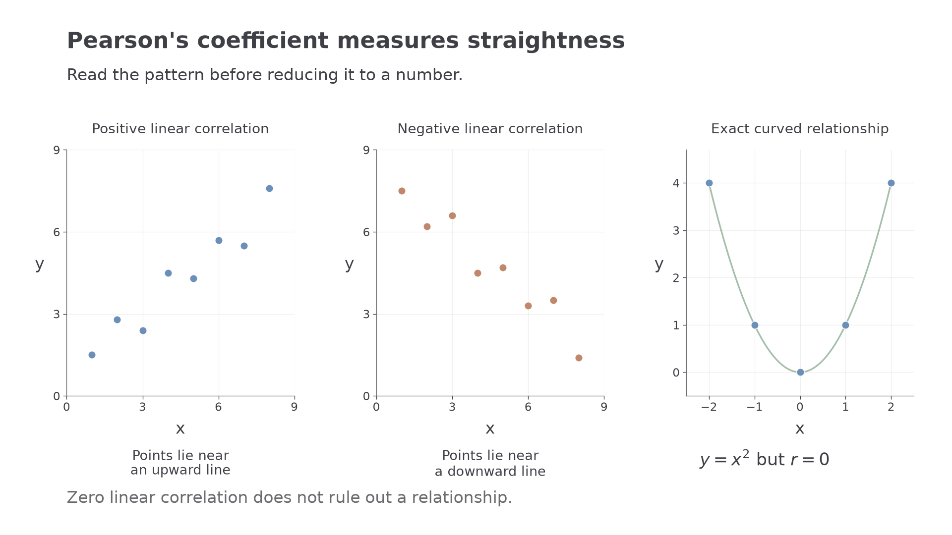
Pearson's coefficient recognises upward and downward straight-line patterns, while a symmetric curved pattern can have zero linear correlation

Here is a useful surprise: the five points $(-2,4)$ , $(-1,1)$ , $(0,0)$ , $(1,1)$ , $(2,4)$ have $r = 0$ , even though every point obeys the exact rule $y = x^2$ . The left-hand downward trend cancels the right-hand upward trend. Zero linear correlation does not mean “no relationship”.

Nor does correlation establish causation. For example, larger plants might both have more leaves and need more water; a positive correlation alone does not show that adding leaves would cause water use to rise. A third variable or the way the sample was selected may help explain an observed pattern. An outlier can also change $r$ substantially, so inspect the scatter diagram before treating one number as the whole story.

Key idea

Pearson's coefficient measures closeness to a straight line. Describe a scatter diagram in terms of its points and the line, and distinguish that description from a claim about cause and effect.

Use the shape as well as the number when deciding what a coefficient says.

Calculating the pmcc

Pearson's coefficient compares how the two variables vary together with how much each varies on its own.

For the five pairs $(1,2)$ , $(2,1)$ , $(3,4)$ , $(4,3)$ , $(5,5)$ , both means are $3$ . A pair lying above both means contributes a positive product $(x_i - \bar{x})(y_i - \bar{y})$ , as does a pair lying below both. A pair above one mean and below the other contributes a negative product. Adding these products measures the tendency to move together.

Product-moment correlation coefficient

For $n$ paired observations, define

\begin{aligned} S_{xx} &= \sum x_i^2 - \frac{(\sum x_i)^2}{n} \\ S_{yy} &= \sum y_i^2 - \frac{(\sum y_i)^2}{n} \\ S_{xy} &= \sum x_i y_i - \frac{\sum x_i\sum y_i}{n} \end{aligned}

Then

r = \frac{S_{xy}}{\sqrt{S_{xx}S_{yy}}}

Both $S_{xx}$ and $S_{yy}$ must be positive. Equivalently, these three sums are $\sum(x_i-\bar{x})^2$ , $\sum(y_i-\bar{y})^2$ and $\sum(x_i-\bar{x})(y_i-\bar{y})$ .

In the formula booklet.

The square-root denominator removes the units and makes the scale of either variable irrelevant. For raw data, enter the paired columns in your calculator's two-variable statistics mode and request $r$ . Calculator functions are expected; you still need to know which coefficient the answer represents. For summaries, keep the three corrected sums separate and retain unrounded values until the end.

Worked example 1: raw paired data

Question. Calculate the pmcc for the following data.

$x$	$1$	$2$	$3$	$4$	$5$
$y$	$2$	$1$	$4$	$3$	$5$

Plan. Keep each column paired, calculate the corrected sums and divide by their geometric mean.

\begin{aligned} \sum x_i &= 15,\quad \sum y_i = 15 && \text{column totals} \\ \sum x_i^2 &= 55,\quad \sum y_i^2 = 55 && \text{squared totals} \\ \sum x_i y_i &= 53 && \text{multiply within pairs} \\ S_{xx} = S_{yy} &= 55 - \frac{15^2}{5} = 10 && \text{correct for the means} \\ S_{xy} &= 53 - \frac{15(15)}{5} = 8 && \text{correct the product sum} \\ r &= \frac{8}{\sqrt{10(10)}} = 0.8 && \text{normalise} \end{aligned}

Why this step? $\sum x_i y_i$ multiplies the two measurements from the same pair; it is not $(\sum x_i)(\sum y_i)$ .

Answer. $r = 0.800$ : the data have positive linear correlation.

Check. A two-variable calculator entry gives $r = 0.8$ . The two reversals in the otherwise rising values of $y$ make a positive coefficient smaller than $1$ sensible.

Worked example 2 changes the presentation: the paired observations are replaced by sufficient summary statistics. The corrected-sum calculation is unchanged.

Worked example 2: summarised paired data

Question. For five pairs of observations,

\sum x_i = 20,\quad \sum y_i = 25,\quad \sum x_i^2 = 90,\quad \sum y_i^2 = 135,\quad \sum x_i y_i = 108

Calculate Pearson's correlation coefficient.

Plan. Use $n = 5$ in each mean correction, then substitute the three corrected sums into the formula for $r$ .

\begin{aligned} S_{xx} &= 90 - \frac{20^2}{5} = 10 && \text{spread in } x \\ S_{yy} &= 135 - \frac{25^2}{5} = 10 && \text{spread in } y \\ S_{xy} &= 108 - \frac{20(25)}{5} = 8 && \text{joint variation} \\ r &= \frac{8}{\sqrt{10(10)}} = 0.800 && \text{substitute} \end{aligned}

Why this step? The formula uses variation about the means; using $108/\sqrt{90(135)}$ would fail to remove those means.

Answer. $r = 0.800$ .

Check. These summaries arise by adding $1$ to every $x$ and $2$ to every $y$ in example 1. The cloud has only moved, so its linear correlation should stay the same.

The sign comes entirely from $S_{xy}$ , because the denominator is positive.

Watch out

Wrong: $r = S_{xy}/(S_{xx}S_{yy})$ . Right: $r = S_{xy}/\sqrt{S_{xx}S_{yy}}$ . Also, if a calculation gives $r = 1.2$ , it cannot be a valid correlation coefficient: check the entries, pairing, squares and brackets.

Now keep the same method but allow the corrected product sum to be negative.

Linear coding and changing units

Changing units or subtracting a convenient baseline is an exact change of scale, so it preserves the straightness of a scatter diagram.

Linear coding

Linear coding replaces a variable by an exact expression $u = a + bx$ , where $a$ and $b$ are constants and $b \ne 0$ . For example, $u = x/100$ converts centimetres to metres. Replacing a person's height by their mass is not linear coding: those measurements do not obey one exact linear rule.

Subtracting the coded mean gives $u_i - \bar{u} = b(x_i - \bar{x})$ : the offset disappears. Similarly, for $v = c + dy$ ,

S_{uu} = b^2S_{xx},\qquad S_{vv} = d^2S_{yy},\qquad S_{uv} = bdS_{xy}

Hence the factors cancel from the coefficient except for their signs. These corrected-sum identities follow from the booklet definitions; they are not separately supplied.

Correlation after linear coding

For non-constant variables and non-zero scales $b$ and $d$ ,

r_{uv} = \frac{bd}{|b||d|}\,r_{xy}

Positive scales leave $r$ unchanged. Reversing exactly one scale reverses its sign; reversing both leaves it unchanged. The magnitude is unchanged in every case.

Not in the formula booklet: learn it.

This is why ordinary unit conversions preserve the coefficient: centimetres and metres both increase in the same direction. A negative scale reflects one axis, so the same strength becomes the opposite direction.

Worked example 3: positive changes of scale

Question. The pmcc between $x$ and $y$ is $0.74$ . Find the pmcc between $u = (x - 20)/5$ and $v = (y + 3)/2$ .

Plan. Identify the signs of the two scale factors; the offsets do not affect deviations from the means.

\begin{aligned} b &= \frac15,\quad d = \frac12 && \text{both positive} \\ r_{uv} &= \frac{(1/5)(1/2)}{|1/5||1/2|}(0.74) && \text{coding rule} \\ &= 0.74 && \text{scale factors cancel} \end{aligned}

Why this step? The constants $-20$ and $+3$ shift the cloud; they cannot alter its straightness or direction.

Answer. The new pmcc is $0.74$ .

Check. Both coded measurements rise when their original measurements rise, so the positive direction is preserved.

Worked example 4 changes only the sign of the scale on $y$ . That reflection reverses the direction while retaining the strength.

Worked example 4: one reversed scale

Question. The pmcc between $x$ and $y$ is $0.74$ . Find the pmcc between $u = (x - 20)/5$ and $w = -(y + 3)/2$ .

Plan. Use the same coding rule with one negative scale factor.

\begin{aligned} b &= \frac15,\quad d = -\frac12 && \text{one negative scale} \\ r_{uw} &= \frac{(1/5)(-1/2)}{|1/5||-1/2|}(0.74) && \text{coding rule} \\ &= -0.74 && \text{sign reverses} \end{aligned}

Why this step? A rise in $y$ becomes a fall in $w$ , so an upward pattern becomes a downward pattern.

Answer. The new pmcc is $-0.74$ .

Check. $w = -v$ compared with example 3, so this is a vertical reflection of exactly the same scatter diagram.

Continue this lesson.

You’re previewing NovaLearn without an account. Create a free account to read the rest.

Create free account

Last Accessed

Pure Core

Statistics

Mechanics

Discrete Mathematics

Additional Pure Mathematics

5.08a–5.08d - Pearson's correlation coefficient and its test

What Pearson's coefficient measures

Calculating the pmcc

Linear coding and changing units

Continue this lesson.

Learn faster with Nova