5.02f–5.02h - The geometric distribution
Model the number of independent trials up to and including the first success. Calculate exact, interval and conditional probabilities, and use the geometric mean and variance to describe waiting in discrete trials.
Counting up to the first success
If a successful trial has probability , the average wait is trials. Is trial therefore the most likely time for the first success? The answer is surprising: trial is the most likely, while the long right tail pulls the average to .
You already know
Multiply probabilities of independent events. A discrete distribution has probability masses at individual values. A mean is a weighted average, and need not be its most likely value.
Imagine repeated independent attempts to pass a fixed automated check. On each attempt, success has the same probability . Record the number of attempts, stopping when the first success occurs: a success immediately gives ; failure then success gives .
Geometric distribution
when is the number of trials up to and including the first success, with independent trials, two outcomes on each trial, and the same success probability , where . Its support is , or just if .
The conditions belong to the experiment, not just its numerical output. Repeated learning attempts may become more successful with practice, violating constant . Sampling without replacement from a small population generally changes . A fixed number of trials with successes counted is a binomial situation instead; a geometric model fixes the stopping rule, not the trial count. These modelling conditions and the stopping convention are not in the formula booklet: learn them.
[DIAGRAM: asset_name: Geometric waiting has a long right tail; asset_slug: h245_5_02_geometric_masses; caption: For Geo(0.2), the first trial is the most likely success time although the mean is 5. A further trial multiplies each probability by 0.8; description: Probability masses for trial numbers 1 to 16 decrease from 0.2 by a factor of 0.8 each time. A dashed vertical line marks the mean at 5. An annotation says that the distribution continues beyond the displayed trials, with remaining probability 0.8 to the power 16]
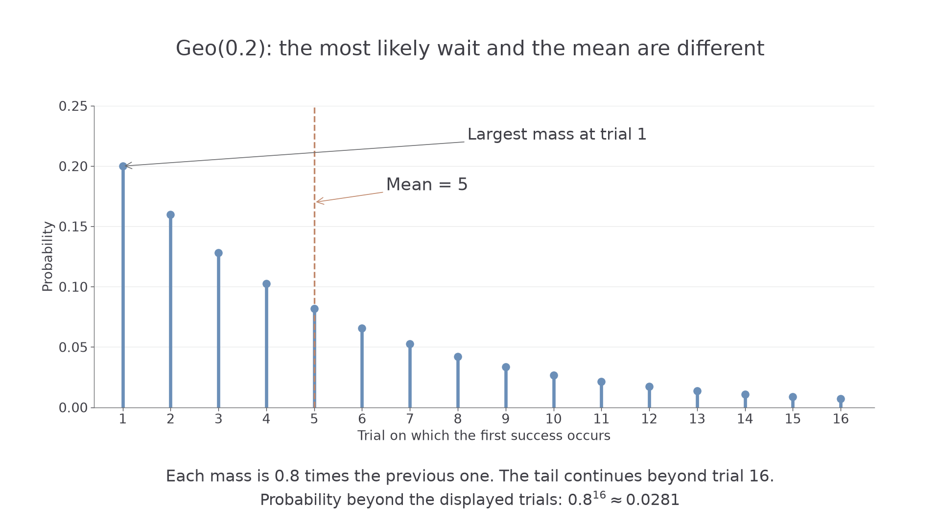
A geometric variable cannot be , because even an immediate success uses one trial. The failure count before success would be , a different variable.
Key idea
Define what is counted before selecting a formula: OCR's geometric variable includes the successful trial.
Check the model by examining its mechanism rather than a verbal resemblance to “waiting”.
The probability of a first success
For the first success to occur on trial , all earlier trials must fail and trial must succeed. There is only one relevant success/failure sequence: failures followed by one success.
Geometric probability mass
If , then for positive integers ,
It is zero outside the support.
In the formula booklet.
The exponent counts failures, not trials. For , the first trial succeeds with certainty, so handle directly; the variable is constant.
Worked example 1: three failures then success
Question. . Find .
Plan. Require three failures followed by success.
Why this step? Trial is successful, so only the preceding trials contribute failure factors.
Answer. , to significant figures.
Check. ; multiplying by three times gives .
Change only the success probability to . Keep the stopping trial fixed so the exponent remains .
Worked example 2: a new success probability
Question. . Find .
Plan. Use failure probability for each of the first three trials.
Why this step? Both factors must change when changes: a higher success probability also lowers the probability of surviving the earlier trials.
Answer. , to significant figures.
Check. The first four masses are , each times its predecessor.
A later first success needs more failures, so for the probabilities strictly decrease with the trial number. This explains why trial is the mode even when the mean is much larger.
Watch out
Wrong: . That sequence has four failures and then success, so it describes . Right: .
Keep the stopping trial fixed and change again.
Tails, intervals and conditional waiting
To wait beyond trial , you need exactly one thing: the first trials all fail. No success factor belongs in that tail probability.
Geometric tails
For and a non-negative integer ,
For a positive integer , .
Not in the formula booklet: learn it.
Continue this lesson.
You’re previewing NovaLearn without an account. Create a free account to read the rest.
Create free account