5.06a - Chi-squared tests for independence | OCR A-Level Further Mathematics A

Decide whether two categorical variables are associated, using observed counts and the counts independence would predict. You will calculate expected frequencies and contributions, combine categories when necessary, choose the degrees of freedom and complete a chi-squared test, including Yates’s correction for a two-by-two table.

Independence and hypotheses

Does a preferred revision format depend on whether a student studies a language? Suppose a random sample gives the following counts.

	Printed notes	Video	Both	Total
Studies a language	$18$	$12$	$10$	$40$
Does not	$12$	$18$	$10$	$40$
Total	$30$	$30$	$20$	$80$

The proportions differ, but random sampling can produce differences even when the population variables are independent. How large must the discrepancy be before it is convincing evidence of association? We will return to these counts after building the test.

You already know

Events $A$ and $B$ are independent when $\mathrm{P}(A\cap B)=\mathrm{P}(A)\mathrm{P}(B)$ . A significance test compares data with a null hypothesis at a chosen significance level; not rejecting a hypothesis does not prove it.

Each person contributes to exactly one cell. The variables are the row category and column category, rather than the individual cells themselves. Treating repeated answers from the same person as independent observations would misrepresent the amount of information.

Contingency table

A contingency table classifies observations by two categorical variables, with one variable defining the rows and the other defining the columns. The entries are observed frequencies, denoted by $O_i$ . The categories within each variable must be mutually exclusive and cover all observations.

For the opening question, write $H_0$ : revision-format preference and language study are independent. The alternative is $H_1$ : revision-format preference and language study are associated.
“No association” is equivalent to “independent”. “No correlation” is unsuitable here: these are categories, not numerical measurements to which a correlation coefficient applies. Hypotheses state population claims, without the words “there is evidence”.

A random sample, independently classified observations and sufficiently large expected frequencies support the chi-squared approximation. A convenient sample of volunteers can still be calculated with, but cannot automatically support conclusions about all students. Association also does not establish cause: taking a language has not been randomly assigned.

Key idea

The test asks whether the differences between observed and independence-based counts are too large to explain plausibly by sampling variation.

Check both the population claim and the way the data were collected before touching the calculator.

Expected frequencies under independence

An expected frequency is the count predicted under the null hypothesis, using the observed row and column totals.

In the opening table, half the sample studies a language and $30/80$ prefer printed notes. Independence predicts a fraction $(40/80)(30/80)$ in both categories, giving $80(40/80)(30/80)=15$ people. Expected counts may be fractional: they are model averages, not a second observed sample.

Expected frequency in a contingency table

For a cell whose row total is $R$ , column total is $C$ , and grand total is $N$ ,

E=\frac{RC}{N}

This fits the null hypothesis of independence using the table's margins.
Not in the formula booklet: learn it.

Calculate from the original margins, not by averaging the observed counts within a row.

Worked example 1: equal row totals

Question. Find the expected frequencies for the opening table.

Plan. Multiply each row total by each column total and divide by $80$ .

\begin{aligned} E_{11}&=\frac{40\times30}{80}=15 &&\text{first row, first column}\\ E_{12}&=\frac{40\times30}{80}=15 &&\text{second column}\\ E_{13}&=\frac{40\times20}{80}=10 &&\text{third column} \end{aligned}

Why this step? Independence gives each row the same column proportions, not necessarily equal column counts.

Answer. The expected table is $\begin{pmatrix}15&15&10\\15&15&10\end{pmatrix}$ , because both row totals are $40$ .

Check. The row totals remain $40,40$ , the column totals remain $30,30,20$ , and all expected frequencies are at least $5$ .

Worked example 2 changes only the balance between the row totals. The same column proportions now produce different expected counts in the two rows.

Worked example 2: unequal row totals

Question. A table has observed counts $\begin{pmatrix}9&6&5\\21&24&15\end{pmatrix}$ . Find its expected frequencies under independence.

Plan. Find the margins before applying $E=RC/N$ .

\begin{aligned} R_1&=20,\quad R_2=60,\quad N=80 &&\text{row totals}\\ (C_1,C_2,C_3)&=(30,30,20) &&\text{column totals}\\ (E_{11},E_{12},E_{13})&=(7.5,7.5,5) &&\text{multiply columns by }20/80\\ (E_{21},E_{22},E_{23})&=(22.5,22.5,15) &&\text{multiply columns by }60/80 \end{aligned}

Why this step? A row containing three times as many people must have three times each expected frequency under independence.

Answer. $\begin{pmatrix}7.5&7.5&5\\22.5&22.5&15\end{pmatrix}$ .

Check. The first expected column totals $7.5+22.5=30$ ; the smallest expected count is exactly $5$ , which meets the condition.

An observed zero is possible under a model with positive expected frequency. Conversely, an observed count of $8$ does not make a cell suitable if its expected count is only $3$ .

Watch out

Wrong: “Every observed count exceeds $5$ , so the condition is satisfied.” Right: check every expected frequency. The threshold is $E_i\ge5$ , not $O_i\ge5$ .

Preserving the margins provides a quick check on a whole expected table.

Contributions and degrees of freedom

A chi-squared statistic adds scaled discrepancies: each cell contributes $(O_i-E_i)^2/E_i$ , so positive and negative differences cannot cancel.

Dividing by $E_i$ matters. A discrepancy of $4$ is more striking beside an expectation of $5$ than beside an expectation of $500$ . Every contribution is non-negative; exact agreement gives zero.

Chi-squared statistic

For a contingency table other than a two-by-two table, with every expected frequency at least $5$ ,

X^2=\sum_i\frac{(O_i-E_i)^2}{E_i}

Under $H_0$ , this is approximately distributed as $\chi^2_\nu$ .
In the formula booklet.

The observed total and fitted margins constrain the cells. In a two-by-three table, once the first two counts in the first row are chosen, its third count is fixed by that row total, and the entire second row is fixed by the column totals. Only two cells vary freely.

Degrees of freedom for independence

For a retained table with $r$ rows and $c$ columns,

\nu=(r-1)(c-1)

Use the dimensions after any combining of rows or columns.
Not in the formula booklet: learn it.

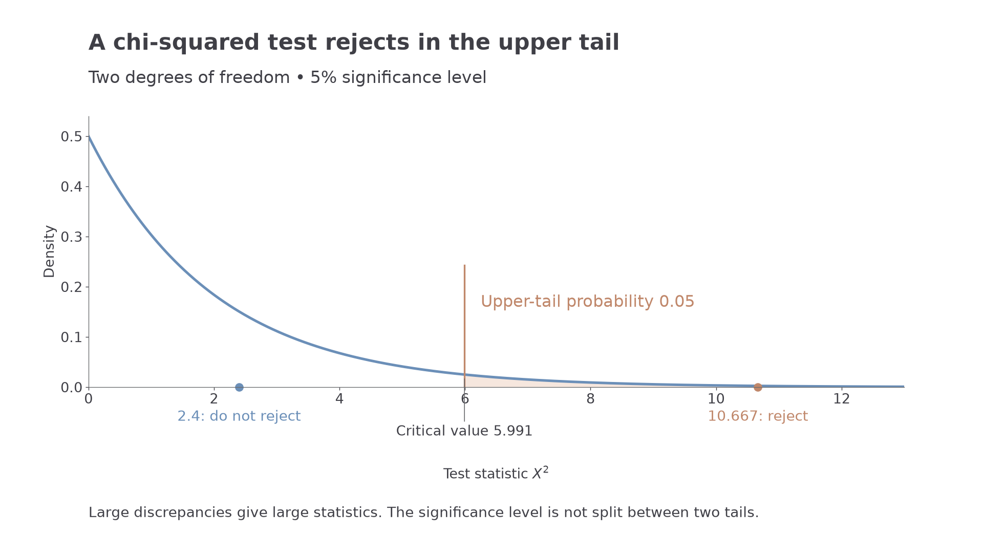
Large values of $X^2$ contradict independence, so the rejection region is always in the upper tail. At the $5\%$ level, choose the critical value with upper-tail probability $0.05$ . The chi-squared critical-value table is in the formula booklet; do not split this probability between two tails.

[DIAGRAM: asset_name: The upper-tail rejection region; asset_slug: h245_5_06_chi_squared_tail; caption: With two degrees of freedom, the upper five per cent begins at 5.991; description: A chi-squared density with two degrees of freedom is drawn above a horizontal statistic axis. The area to the right of the vertical line at 5.991 is shaded pale clay and labelled upper-tail probability 0.05. A marker at 2.4 lies to the left of the line and a marker at 10.667 lies to its right]
With two degrees of freedom, the upper five per cent begins at 5.991

Worked example 3: complete the opening test

Question. Test the opening revision-format data at the $5\%$ significance level. Assume independent observations from a random sample.

Plan. Use the expected counts $(15,15,10)$ in each row, add all six contributions and compare with $\chi^2_2$ .

The hypotheses are those stated in the first part.

\begin{aligned} X^2&=\frac{(18-15)^2}{15}+\frac{(12-15)^2}{15}+0 +\frac{(12-15)^2}{15}+\frac{(18-15)^2}{15}+0 &&\text{all six cells}\\ &=4\times\frac9{15}=2.4 &&\text{sum contributions}\\ \nu&=(2-1)(3-1)=2 &&\text{retained dimensions}\\ 2.4&<5.991 &&\text{upper }5\%\text{ critical value} \end{aligned}

Why this step? The small statistic says the observed differences are not unusually large under independence; different observed proportions alone are insufficient.

Answer. Do not reject $H_0$ . At the $5\%$ level there is insufficient evidence of association between revision-format preference and language study.

Check. Both $10$ -count cells agree exactly with expectation, and all four other contributions are $0.6$ .

Worked example 4 changes only the allocation of counts within the same margins. The expected counts and critical value stay fixed, isolating the effect of greater discrepancy.

Worked example 4: stronger disagreement with the same margins

Question. Another independent random sample gives $\begin{pmatrix}22&10&8\\8&20&12\end{pmatrix}$ for the same two variables. Test for association at the $5\%$ level.

Plan. Keep the same hypotheses and expected table, then recalculate the contributions.

\begin{aligned} X^2&=2\left(\frac{7^2}{15}+\frac{5^2}{15}+\frac{2^2}{10}\right) &&\text{equal squared differences in both rows}\\ &=\frac{32}{3}=10.666\ldots &&\text{sum without early rounding}\\ \nu&=2,\qquad 10.666\ldots>5.991 &&\text{compare with the same critical value} \end{aligned}

Why this step? The margins determine expectation; the cells' departures from that expectation determine evidence against independence.

Answer. Reject $H_0$ . There is sufficient evidence, at the $5\%$ level, of association between revision-format preference and language study.

Check. The first column alone contributes $2(49/15)>6$ , already beyond the critical value; the full sum must be larger.

Continue this lesson.

You’re previewing NovaLearn without an account. Create a free account to read the rest.

Create free account

Last Accessed

Pure Core

Statistics

Mechanics

Discrete Mathematics

Additional Pure Mathematics

5.06a - Chi-squared tests for independence

Independence and hypotheses

Expected frequencies under independence

Contributions and degrees of freedom

Continue this lesson.

Learn faster with Nova