5.02m, 5.02n - Poisson mean, variance and sums
Use the equality of Poisson mean and variance, combine independent Poisson counts, and recognise when that addition rule cannot be used. Distinguish exact distribution properties from the approximate patterns expected in a finite sample.
One parameter for location and spread
If two counters each record Poisson events, can you add their readings and still use a Poisson model? The answer depends on how the counters are related. First notice a special feature of each individual count: its mean and variance are exactly equal.
You already know
counts events in a specified interval, using the interval's average count as parameter. Its mass is . Variance equals , and standard deviation is the square root of variance.
The same parameter controls both the location and the squared spread. Doubling a Poisson interval's parameter doubles its variance, while its standard deviation grows by a factor of . Relative variability, measured by standard deviation divided by mean, therefore decreases as counts grow.
Poisson moments
For ,
Consequently its standard deviation is .
In the formula booklet.
The equality concerns the numerical mean and variance. If a count is recorded in units of events, the variance has squared units; it is not a statement that the physical units are identical.
Worked example 1: recovering a second moment
Question. . Find , and .
Plan. Read off the mean and variance, then rearrange the variance identity.
Why this step? Squaring the mean gives , which is smaller than the second moment by exactly the variance.
Answer. Mean , variance , second moment .
Check. , recovering the variance.
Change only the parameter from to . The method stays the same, but the second moment does not increase merely by .
Worked example 2: a larger count parameter
Question. . Find , and .
Plan. Use the Poisson moments and add the squared mean to the variance.
Why this step? The location contribution is the square of the new mean, so both terms change.
Answer. Mean , variance , second moment .
Check. ; the standard deviation is , not .
These exact identities can rule out proposed population parameters. A variable with exact mean and exact variance is not Poisson. By contrast, a sample mean of and sample variance of need not be exactly equal: their closeness is consistent with a Poisson model, but does not prove one. Substantially different sample summaries may cast doubt on the model; use a qualified conclusion and consider its assumptions too.
Watch out
Wrong: “The sample mean and variance differ, so the distribution cannot be Poisson.” Random samples fluctuate. Exact equality is a population property, not an identity for every realised sample.
A second moment links this lesson to the general distribution calculations.
Adding independent Poisson counts
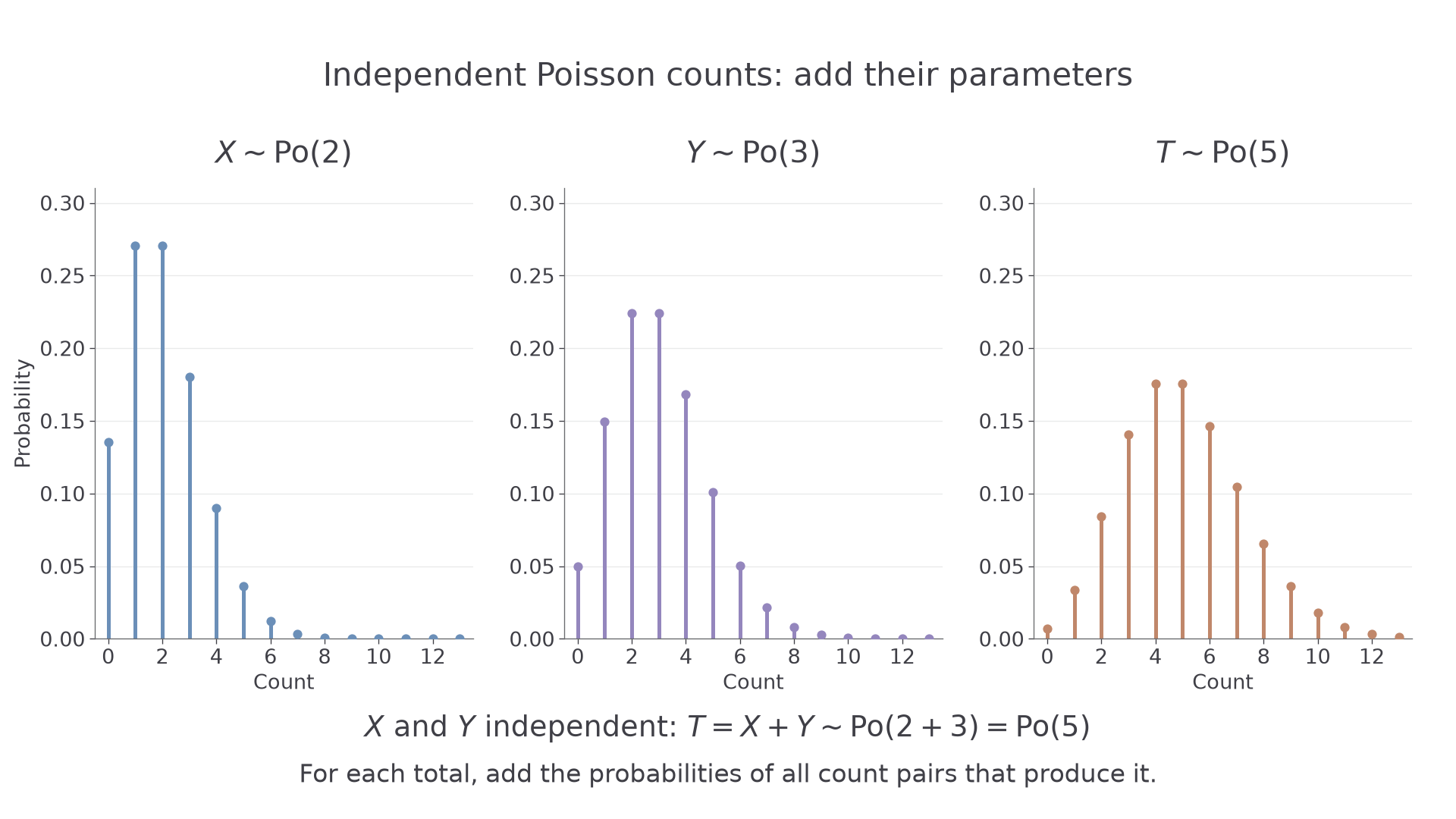
Suppose one sensor counts events of one kind and another counts a different kind. If the two counts are independent and both are Poisson, the total is Poisson too: simply add their parameters.
Sum of independent Poisson variables
If and , and are independent, then
More generally, the sum of mutually independent Poisson variables is Poisson with parameter equal to the sum of their parameters.
Not in the formula booklet: learn it.
The statement concerns independent random variables, rather than merely independent event occurrences within each separate model. To obtain a total of , for example, possible count pairs are . Multiply within each pair using independence, then add their probabilities. The resulting masses follow the Poisson formula with the combined parameter.
[DIAGRAM: asset_name: Independent Poisson masses combine; asset_slug: h245_5_02_poisson_sum; caption: The independent counts X with Po(2) and Y with Po(3) combine to a Po(5) count. The total distribution is obtained by adding probabilities of count pairs with the same total; description: Three probability-mass plots show Po(2), Po(3) and Po(5) with common integer count axes. The first two are blue and lavender; the total is clay. A line of text states independent X and Y, T = X + Y, parameter 2 + 3 = 5]
Do not add observed counts and call the result a parameter. The total parameter comes from the model's average counts over the specified intervals.
Continue this lesson.
You’re previewing NovaLearn without an account. Create a free account to read the rest.
Create free account