4.10b - Modelling with differential equations
A differential equation turns a statement about rates or forces into a prediction. You will construct and interpret models in kinematics and other contexts, solve suitable first order models, and distinguish a model you can formulate from one you can solve analytically.
Variable force and motion
Can a constant driving force produce a speed limit? It can when resistance grows with velocity. To understand that result, first translate a simpler changing force into an equation for motion.
You already know
For a particle of constant mass, Newton's second law is resultant force equals mass times acceleration. Choose a positive direction before assigning force and velocity signs. Integrating acceleration gives velocity; integrating velocity gives displacement.
Let be the signed displacement in the chosen direction, measured at time . A dot means differentiation with respect to time; it does not mean multiplication.
Kinematics and Newton's second law
For constant mass , in a fixed direction,
and
The force and velocity are signed components along that direction.
Not in the formula booklet: learn it.
When the force changes, the constant-acceleration formulae do not apply. Construct the derivative equation and integrate it instead.
Worked example 1: a force proportional to time
Question. A particle of mass moves along a straight line. Its resultant force at time seconds is in the positive direction. Initially and . Find and in terms of .
Plan. Use Newton's second law, integrate for velocity and displacement, and use each initial condition.
Why this step? The given force is the resultant, so no extra force is added to it; divide by the mass to obtain acceleration.
Answer. and , for .
Check. Differentiating gives and , and both initial conditions hold.
Add only a constant opposing contribution of to the resultant force. Its sign must survive both integrations.
Worked example 2: a signed changing resultant
Question. The same particle now has resultant force , measured positively in the same direction, with the same initial conditions. Find and .
Plan. Retain the negative force term when forming acceleration, then integrate twice.
Why this step? A negative resultant means negative acceleration, not automatically negative velocity; the initial motion still matters.
Answer. and , for .
Check. At , acceleration is while velocity is , consistent with initially slowing down.
Signs encode the direction of the force; taking its magnitude too early changes the model.
Watch out
Wrong: , replacing the signed resultant by its size. Right: throughout the model's stated interval.
Change the constant opposing term once more, and keep velocity signed.
Velocity dependent resistance
A force depending on velocity makes the unknown function appear on both sides of Newton's law. With resistance proportional to velocity, the resulting equation is linear and the integrating factor method applies.
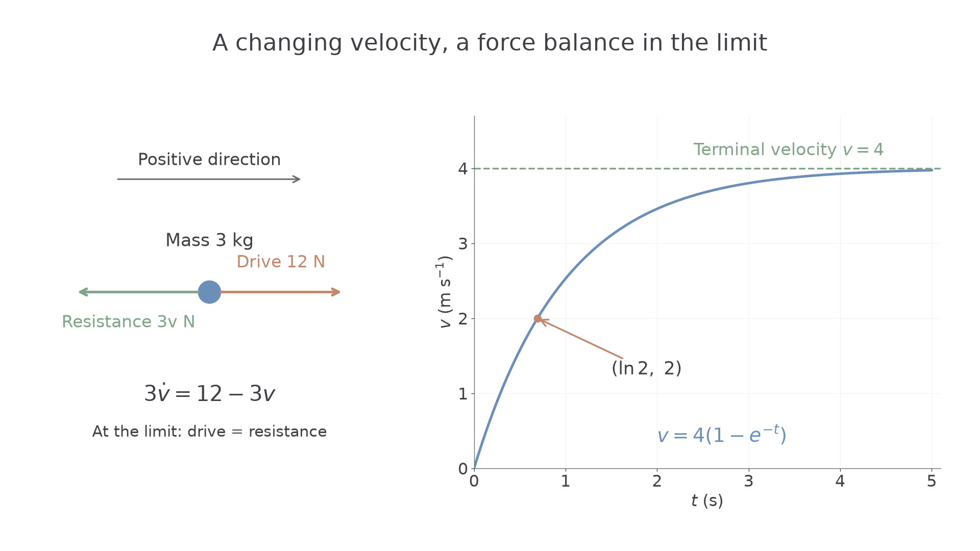
Suppose a constant drive acts positively and a resistive force has signed component , with . The minus sign makes resistance oppose the motion. Newton's law is . At a steady velocity, , so the drive and resistance balance.
Terminal velocity
A terminal velocity is a limiting steady velocity approached as the resultant force tends to zero. In the model , it is . For vertical falling motion with downward positive, the corresponding model is , giving terminal velocity .
Terminal velocity is a prediction of the force law. It is not an extra force to add to the equation.
These terminal-velocity results are not in the formula booklet; obtain them by setting the resultant force to zero.
[DIAGRAM: asset_name: Drive and resistance approach a balance; asset_slug: h245_4_10_terminal_velocity; caption: For a 3 kg particle with 12 N drive and resistance 3v N, velocity rises towards 4 metres per second while acceleration tends to zero; description: Left panel shows a particle with a rightward arrow labelled drive 12 N, a leftward arrow labelled resistance 3v N, and a rightward positive direction. Right panel plots v = 4(1 - exp(-t)) for t from 0 to 5, starting at the origin and approaching a dashed horizontal terminal line v = 4. The half-terminal point (ln 2, 2) is marked and labelled.]
Worked example 3: approaching terminal velocity
Question. A particle starts from rest on a horizontal line. A constant drive of acts positively and the resistance has signed component , where is in . Find and its limiting value.
Plan. Resolve forces, divide by the mass and solve the linear equation with its initial condition.
Why this step? Resistance is part of the resultant, so the equation is , rather than .
Answer. , tending to as .
Check. . At the limiting velocity, resistance is , balancing the drive.
Change only the driving force from to . The rate of approach stays the same, but the limiting velocity changes.
Worked example 4: changing the drive
Question. The same particle, starting from rest, has drive and the same resistance law. Find its velocity and the time to reach half its terminal velocity.
Plan. Solve the new linear equation, then set the velocity equal to half its limiting value.
Why this step? Half-terminal velocity is half the new limit , rather than half the previous limit .
Answer. ; the required time is .
Check. At , , so .
In fact, the first particle also reaches half its terminal velocity at . Increasing the drive raises both velocities in the same proportion; it does not change the time needed to complete the same fraction of the approach in this linear model. This conclusion depends on the assumed resistance law.
Continue this lesson.
You’re previewing NovaLearn without an account. Create a free account to read the rest.
Create free account