5.05d - Confidence intervals for a population mean | OCR A-Level Further Mathematics A

Estimate an unknown population mean by an interval that reflects sampling uncertainty. You will construct normal confidence intervals with a known or estimated variance, interpret the confidence level correctly, and work backwards from a desired precision to a sample size.

An interval from a normal sample mean

A random sample gives a mean reading of $50$ . How wide should an interval around $50$ be, and how many readings would reduce its margin of error to $0.5$ ? A bare mean conceals uncertainty; an interval displays it.

Suppose $16$ independent readings come from a normal population with known standard deviation $4$ . Their mean has standard error $4/\sqrt{16}=1$ . About $95\%$ of repeated sample means lie within $1.96$ standard errors of the population mean. Reversing that statement gives intervals around those sample means which contain the population mean in about $95\%$ of repetitions.

You already know

For a normal population of mean $\mu$ and known variance $\sigma^2$ , the independent sample mean is exactly $\mathrm{N}(\mu,\sigma^2/n)$ . The booklet supplies this distribution, its standardisation and normal percentage points. The interval is centred on the observed $\overline x$ , whereas a hypothesis-test null distribution is centred on $\mu_0$ .

The central normal probability explains both the multiplier and the two endpoints. If $z=z_{1-\alpha/2}$ , then

\mathrm{P}\left(-z\le\frac{\overline X-\mu}{\sigma/\sqrt n}\le z\right)=1-\alpha

Rearranging the inequalities puts $\mu$ between $\overline X-z\sigma/\sqrt n$ and $\overline X+z\sigma/\sqrt n$ . The endpoints are random before sampling; after sampling, they are calculated numbers.

Confidence interval and margin of error

A confidence interval for a population mean is an interval calculated from sample data using a procedure with a stated long-run coverage rate. A $100(1-\alpha)\%$ procedure contains the true mean in a proportion $1-\alpha$ of repetitions under the model. For a symmetric interval $\overline x\pm m$ , the margin of error $m$ is its half-width; its full width is $2m$ .

For a known normal population variance, the sampling model gives an exact interval procedure. The decimal multipliers in the table are rounded normal percentage points.

Normal confidence interval with known variance

For a random independent sample of size $n$ from a normal population with known, given or assumed variance $\sigma^2$ , a $100(1-\alpha)\%$ confidence interval for $\mu$ is

\left(\overline x-z_{1-\alpha/2}\frac{\sigma}{\sqrt n}, \ \overline x+z_{1-\alpha/2}\frac{\sigma}{\sqrt n}\right)

Here $\mathrm{P}(Z\le z_{1-\alpha/2})=1-\alpha/2$ , with $Z\sim\mathrm{N}(0,1)$ .

Confidence level	Upper cumulative probability	Multiplier
$90\%$	$0.95$	$1.64485\ldots$
$95\%$	$0.975$	$1.95996\ldots$
$99\%$	$0.995$	$2.57583\ldots$

The normal percentage points are supplied; the interval formula itself is not printed.

Not in the formula booklet: learn it.

Subtract and add the same margin. A quick midpoint check catches a surprising number of slips.

Worked example 1: a ninety-five percent interval

Question. Readings are normally distributed with known variance $16$ . A random independent sample of $16$ readings has mean $50$ . Find a $95\%$ confidence interval for the population mean, giving endpoints to $2$ decimal places.

Plan. Calculate the standard error, multiply it by the central $95\%$ normal multiplier, and place that margin on either side of the observed mean.

\begin{aligned} \mathrm{se}(\overline X)&=\frac4{\sqrt{16}}=1 &&\text{known variance}\\ m&=1.95996\ldots(1)=1.95996\ldots &&\text{two }2.5\%\text{ tails}\\ \text{interval}&=(50-m,50+m) &&\text{centre on the data}\\ &=(48.040036\ldots,51.959964\ldots) &&\text{calculate endpoints} \end{aligned}

Why this step? $95\%$ is the central probability, so use cumulative probability $0.975$ for the positive endpoint, not $0.95$ .

Answer. The $95\%$ confidence interval is $(48.04,51.96)$ .

Check. The midpoint is $50$ , and the half-width is approximately $1.96$ , which is nearly two standard errors.

Worked example 2 changes only the confidence level. More confidence requires a wider interval when the data stay the same.

Worked example 2: increasing the confidence level

Question. For the same sample, with $n=16$ , $\overline x=50$ and known population variance $16$ , find a $99\%$ confidence interval for the population mean. Give endpoints to $2$ decimal places.

Plan. Keep the standard error and sample mean, but use the central $99\%$ multiplier.

\begin{aligned} \mathrm{se}(\overline X)&=1 &&\text{same data and variance}\\ m&=2.57583\ldots(1)=2.57583\ldots &&\text{two }0.5\%\text{ tails}\\ \text{interval}&=(50-2.57583\ldots,50+2.57583\ldots) &&\text{same centre}\\ &=(47.424171\ldots,52.575829\ldots) &&\text{calculate} \end{aligned}

Why this step? To include the fixed population mean more often across repeated samples, the procedure must allow a larger range of sampling fluctuations.

Answer. The $99\%$ confidence interval is $(47.42,52.58)$ .

Check. It contains the $95\%$ interval and has the same midpoint. Greater confidence has not made the estimate more precise.

The two endpoints are estimates of a plausible range for one population mean. They are not lower and upper limits for individual readings.

Watch out

Wrong: using $\sigma$ , rather than $\sigma/\sqrt n$ , as the uncertainty around $\overline x$ . Right: construct an interval for the mean using its standard error. An interval intended to cover individual observations answers a different question.

Keep the requested confidence level and endpoint accuracy distinct: the former chooses a multiplier, and the latter controls rounding.

Large-sample intervals with known or estimated variance

A normal population is not essential if the independent sample is sufficiently large. The central limit theorem gives an approximately normal distribution for the sample mean, so the same interval construction becomes approximate.

There are two distinct variance cases. If the population variance is supplied, use it directly. If it is unknown, estimate it from the sample with the unbiased $s^2$ formula, then use $s/\sqrt n$ . Random independent observations and finite population variance are still required.

Large-sample confidence intervals

For a sufficiently large random independent sample from a population with mean $\mu$ and finite variance, use the approximate interval

\overline x\pm z_{1-\alpha/2}\frac{\sigma}{\sqrt n}

when the population variance $\sigma^2$ is known, given or assumed. When it is unknown, use

\overline x\pm z_{1-\alpha/2}\frac{s}{\sqrt n}, \qquad s^2=\frac{\sum x^2-(\sum x)^2/n}{n-1}

The central limit theorem and the unbiased estimate are supplied in the booklet, but these interval procedures are not printed. An estimated variance makes the normal procedure approximate even if the original population is normal.

Not in the formula booklet: learn it.

The approximate interval has the same centre-plus-or-minus-margin structure. Give the reason for normality and make clear whether its variance is known or estimated.

Worked example 3: an unspecified population with known variance

Question. A population has unspecified distribution and known variance $64$ . A random independent sample of $64$ observations has mean $80$ . Find an approximate $95\%$ confidence interval for the population mean, giving endpoints to $2$ decimal places.

Plan. Use the central limit theorem for the sample mean and the supplied population variance for its standard error.

\begin{aligned} \overline X&\approx\mathrm{N}(\mu,64/64) &&\text{large independent sample}\\ \mathrm{se}(\overline X)&=\sqrt{64/64}=1 &&\text{known variance}\\ m&=1.95996\ldots(1) &&\text{central }95\%\\ \text{interval}&=(80-m,80+m) &&\text{observed centre} \end{aligned}

Why this step? The central limit theorem changes the distributional shape you may use for the mean. It does not turn the population distribution into a normal distribution.

Answer. The approximate $95\%$ confidence interval is $(78.04,81.96)$ .

Check. The half-width is $1.96$ to $2$ decimal places, and no $64/63$ correction has been applied to the known population variance.

Worked example 4 changes only the status of the variance: it is now unknown and must be estimated. These sample summaries happen to give the same numerical variance, but the additional source of approximation matters.

Worked example 4: estimating the variance from summaries

Question. A population has unspecified distribution and unknown variance. A random independent sample of $64$ observations gives $\sum x=5120$ and $\sum x^2=413632$ . Find an approximate $95\%$ confidence interval for its mean, giving endpoints to $2$ decimal places.

Plan. Estimate the mean and population variance, then insert the estimated standard error in the large-sample interval.

\begin{aligned} \overline x&=\frac{5120}{64}=80 &&\text{sample mean}\\ s^2&=\frac{413632-5120^2/64}{63}=64 &&\text{unbiased variance estimate}\\ \widehat{\mathrm{se}}(\overline X)&=\sqrt{64/64}=1 &&\text{estimated mean spread}\\ \text{interval}&=80\pm1.95996\ldots(1) &&\text{large-sample normal interval} \end{aligned}

Why this step? Divide by $n-1$ when estimating the population variance, then divide that estimate by $n$ when estimating the variance of the mean. The two divisions serve different purposes.

Answer. The approximate $95\%$ confidence interval is $(78.04,81.96)$ .

Check. The squared-deviation total is $4032$ ; $4032/63=64$ , whereas dividing it by $64$ would give the uncorrected variance $63$ .

All three permitted cases are now covered: a normal population with known variance, a large sample with known variance, and a large sample with unknown variance. A small sample with unknown variance does not become eligible for this normal procedure merely because you can calculate $s^2$ .

Watch out

Wrong: “The data are a sample, so correct the supplied population variance by $n/(n-1)$ .” Right: use a supplied population variance as it stands. The correction belongs only to an uncorrected variance calculated from sample data.

The final calculation changes the confidence level as well as using a fresh set of summary statistics.

What the confidence level describes

A $95\%$ confidence procedure is a statement about repeated intervals, not about repeated changes in the population mean. The true $\mu$ is fixed; different random samples produce different centres and endpoints.

[DIAGRAM: asset_name: Repeated confidence intervals and a fixed population mean; asset_slug: h245_5_05_interval_coverage; caption: Different samples move the interval while the true population mean stays fixed; description: Twenty horizontal intervals of equal half-width 1.960 with different sample-mean centres, compared with a fixed vertical population-mean line at 50. Nineteen cross the line and one misses it. The caption states that this is one possible set of intervals and that 95 percent coverage is a long-run rate, not a promise of exactly nineteen successes in every twenty samples.]
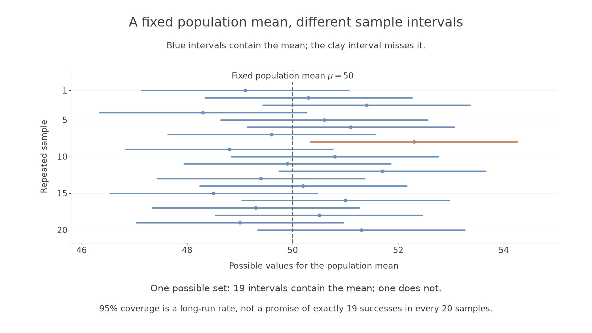
Different samples move the interval while the true population mean stays fixed

The picture shows one possible collection with $19$ intervals containing $\mu$ and one missing it. Another collection of $20$ could give $18$ , $20$ , or another number of successful intervals. The confidence level does not promise an exact count in every small batch.

Once you have calculated a particular interval, it either contains $\mu$ or it does not. In this interpretation, $\mu$ is not a random draw that has a $95\%$ probability of falling into your now-fixed interval. Instead say: “We are $95\%$ confident that the population mean lies between these endpoints”, and understand that the confidence comes from the procedure's coverage rate.

Continue this lesson.

You’re previewing NovaLearn without an account. Create a free account to read the rest.

Create free account

Last Accessed

Pure Core

Statistics

Mechanics

Discrete Mathematics

Additional Pure Mathematics

5.05d - Confidence intervals for a population mean

An interval from a normal sample mean

Large-sample intervals with known or estimated variance

What the confidence level describes

Continue this lesson.

Learn faster with Nova