5.09a–5.09e - Least squares regression lines | OCR A-Level Further Mathematics A

A regression line turns a scatter diagram into a prediction, but the direction of prediction matters. Learn how least squares chooses the line, calculate it from raw or summarised data, translate it under linear coding and decide how much confidence a prediction deserves.

Variables and vertical residuals

Can the best line for predicting $y$ from $x$ simply be rearranged to give the best prediction of $x$ from $y$ ? Start with just three observed pairs: $(1, 1)$ , $(2, 3)$ and $(3, 2)$ . A sensible rising line is $y = 1 + 0.5x$ . Later you will find that the line for predicting in the opposite direction is different. “Best” needs a direction before it has a meaning.

You already know

A scatter diagram displays paired observations. Pearson's coefficient $r = S_{xy}/\sqrt{S_{xx}S_{yy}}$ measures their linear correlation; swapping the variables leaves $r$ unchanged. Correlation alone does not establish cause and effect.

An experiment may choose that direction for you. If you set a water bath's temperature and record how long a reaction takes, temperature is the controlled input and reaction time is the response. If you measure people's hand lengths and foot lengths, neither measurement is controlled. You can still nominate one as a predictor, but the choice does not make it a cause of the other.

Independent and dependent variables

An independent, or controlled, variable is the variable whose values are set in an experiment. The dependent, or response, variable is the measured response. In observational data neither variable need be independent in this sense. This use of “independent” does not mean independence of random variables.

For prediction of $y$ , compare the observed $y$ -value with the line's prediction at the same $x$ . The signed difference is positive above the line and negative below it.

Residual and least squares

For a proposed line $y = a + bx$ , the residual at $(x_i, y_i)$ is $e_i = y_i - (a + bx_i)$ . The least squares regression line of $y$ on $x$ is the line that minimises the sum of the squared vertical residuals, $\sum e_i^2$ .

Squaring prevents positive and negative residuals from cancelling and gives greater weight to a large miss. The distances are vertical: perpendicular distances to the line solve a different problem.

[DIAGRAM: asset_name: Comparing squared vertical residuals; asset_slug: h245_5_09_vertical_residuals; caption: Both lines have residuals summing to zero, but line A has the smaller sum of squared vertical residuals; description: Two scatter diagrams display the points (1,1), (2,3), (3,2). Left line y=1+0.5x has residuals -0.5,1,-0.5 and squared sum 1.5. Right line y=2 has residuals -1,1,0 and squared sum 2. Sage segments show vertical residuals.]
Both lines have residuals summing to zero, but line A has the smaller sum of squared vertical residuals

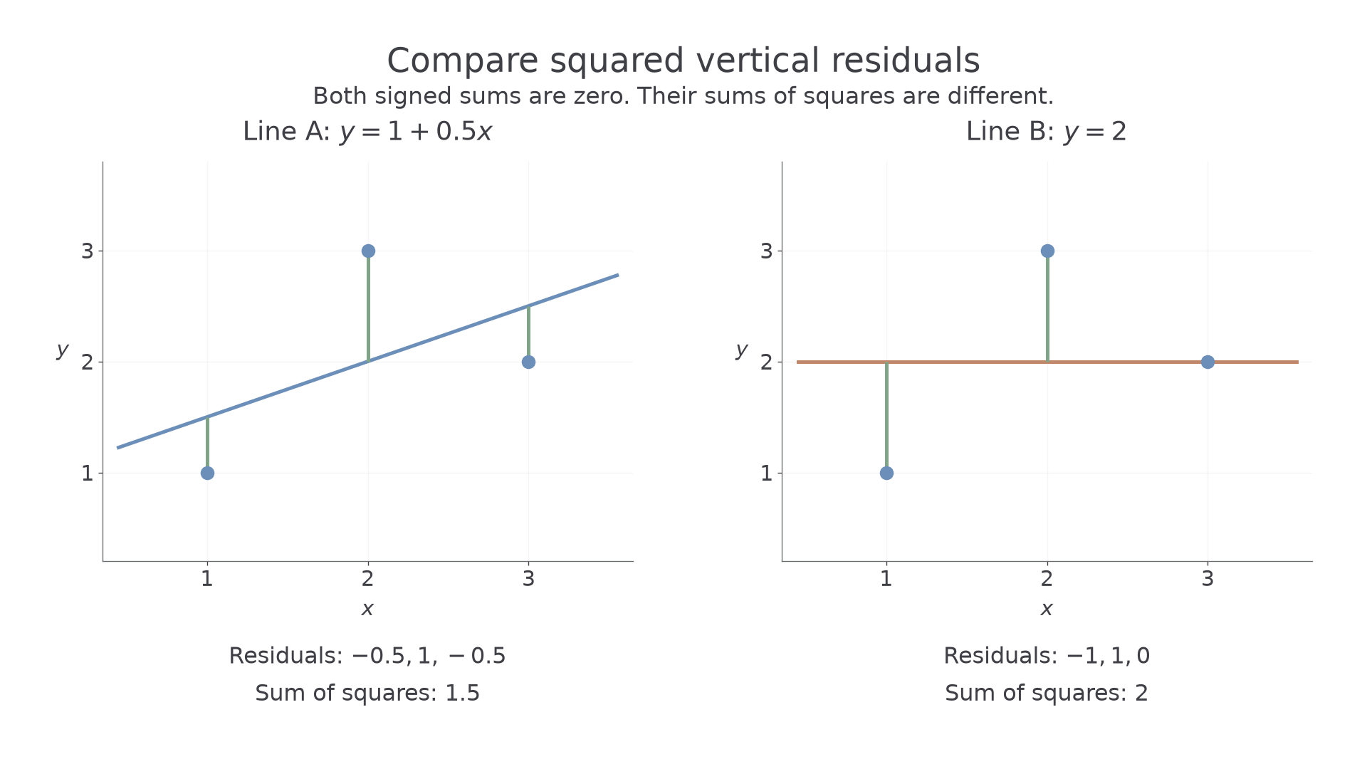
For line A, the squared sum is $(-0.5)^2 + 1^2 + (-0.5)^2 = 1.5$ . For line B, it is $(-1)^2 + 1^2 + 0^2 = 2$ . Line A wins this comparison. Its residuals still need not be small for every individual observation.

Key idea

Predicting $y$ means minimising squared errors in $y$ , measured vertically. A small signed total is not the least squares criterion.

This distinction is what the following calculation overlooks.

Calculating the regression line

The least squares calculation uses the same centred sums as correlation, but a regression coefficient is a gradient with units, rather than a unit-free measure of strength.

You already know

For $n$ pairs, $\bar{x} = \sum x_i/n$ , $\bar{y} = \sum y_i/n$ , $S_{xx} = \sum x_i^2 - (\sum x_i)^2/n$ and $S_{xy} = \sum x_i y_i - (\sum x_i)(\sum y_i)/n$ . These centred-sum formulae are in the formula booklet.

When $S_{xx} > 0$ , the predictor takes more than one value, so its variation can identify a gradient. If all the $x$ -values are equal, there is no uniquely determined regression gradient of $y$ on $x$ .

Regression of y on x

For $S_{xx} > 0$ , the least squares line is

\begin{aligned} y &= a + bx \\ b &= \frac{S_{xy}}{S_{xx}} \\ a &= \bar{y} - b\bar{x} \end{aligned}

In the formula booklet.

Choose the denominator by naming the predictor: “ $y$ on $x$ ” puts $S_{xx}$ underneath. The intercept then makes the line pass through the mean point $(\bar{x}, \bar{y})$ , because $a + b\bar{x} = \bar{y}$ . This mean-point property is not printed separately in the formula booklet: learn it. Remarkably, it holds even when the scatter is curved and a straight-line model would be poor.

Worked example 1: fitting raw data

Question. Calculate the regression line of $y$ on $x$ for these observations.

$x$	$1$	$2$	$3$	$4$	$5$
$y$	$2$	$4$	$5$	$4$	$7$

Plan. Obtain the sums, calculate the two centred sums, then find the gradient and intercept.

\begin{aligned} n &= 5,\quad \sum x_i = 15,\quad \sum y_i = 22 && \text{count and total} \\ \sum x_i^2 &= 55,\quad \sum x_i y_i = 76 && \text{square and multiply pairs} \\ \bar{x} &= 3,\quad \bar{y} = 4.4 && \text{divide totals by } 5 \\ S_{xx} &= 55 - \frac{15^2}{5} = 10 && \text{centre the predictor} \\ S_{xy} &= 76 - \frac{15 \times 22}{5} = 10 && \text{centre the products} \\ b &= \frac{10}{10} = 1 && \text{divide by } S_{xx} \\ a &= 4.4 - 1 \times 3 = 1.4 && \text{use the mean point} \end{aligned}

Why this step? The products must pair each $x_i$ with its own $y_i$ ; multiplying the two totals would discard the association between the measurements.

Answer. $y = 1.4 + x$

Check. At $x = \bar{x} = 3$ , the line gives $y = 4.4 = \bar{y}$ . Its residuals are $-0.4$ , $0.6$ , $0.6$ , $-1.4$ , $0.6$ , whose sum is zero.

Worked example 2 changes how the data are supplied: summaries replace the list of pairs. The calculation is identical, but you must distinguish the sum of the squares from the square of the sum.

Worked example 2: fitting summarised data

Question. Six paired observations have

\sum x_i = 30,\quad \sum y_i = 54,\quad \sum x_i^2 = 170,\quad \sum x_i y_i = 308

Calculate the regression line of $y$ on $x$ .

Plan. Recover the means and centred sums, then substitute into the regression formulae.

\begin{aligned} \bar{x} &= \frac{30}{6} = 5,\quad \bar{y} = \frac{54}{6} = 9 && \text{calculate means} \\ S_{xx} &= 170 - \frac{30^2}{6} = 20 && \text{subtract the mean correction} \\ S_{xy} &= 308 - \frac{30 \times 54}{6} = 38 && \text{centre the products} \\ b &= \frac{38}{20} = 1.9 && \text{regress } y \text{ on } x \\ a &= 9 - 1.9 \times 5 = -0.5 && \text{use the mean point} \end{aligned}

Why this step? $\sum x_i^2 = 170$ is already supplied; it is not $(\sum x_i)^2 = 900$ .

Answer. $y = -0.5 + 1.9x$

Check. Substitution of the mean predictor $x = 5$ gives the mean response $y = 9$ .

A correlation coefficient and a regression gradient share a numerator but have different denominators and different jobs.

Watch out

Wrong: $b = r$ . Correlation divides by $\sqrt{S_{xx}S_{yy}}$ ; the gradient for $y$ on $x$ divides by $S_{xx}$ . Right: $b = S_{xy}/S_{xx}$ . A regression gradient can exceed $1$ , and its size depends on the measurement units.

For a routine “Calculate the equation” question, show enough working to identify your gradient and intercept; these are the two numerical results the equation needs.

The two prediction directions

When neither variable is controlled, you may want to predict either one from the other, and each direction has its own least squares line.

For $x$ on $y$ , the response is $x$ , so residuals run horizontally on the usual scatter diagram. Relabel the formula in the booklet: the predictor's centred sum is now $S_{yy}$ .

Regression of x on y

For $S_{yy} > 0$ , with neither variable controlled, the least squares line for predicting $x$ is

x - \bar{x} = \frac{S_{xy}}{S_{yy}}(y - \bar{y})

This is the booklet's regression rule with the variables interchanged.
Not in the formula booklet: learn it.

Both centred equations are satisfied by $(\bar{x}, \bar{y})$ . If the lines are distinct, that is their intersection; if the observations lie exactly on a non-horizontal, non-vertical line, the two lines coincide. In particular, the original three points have mean point $(2, 2)$ , and the two fitted lines meet there.

[DIAGRAM: asset_name: Two regression directions through the mean point; asset_slug: h245_5_09_two_regression_lines; caption: For the same three points, the two least squares lines meet at the mean point but give different predictions away from it; description: The points (1,1), (2,3), (3,2) appear on a scatter diagram. The blue y-on-x line y=1+0.5x and clay x-on-y line x=1+0.5y cross at the sage mean point (2,2). Labels connect each line to its vertical or horizontal squared-residual criterion.]
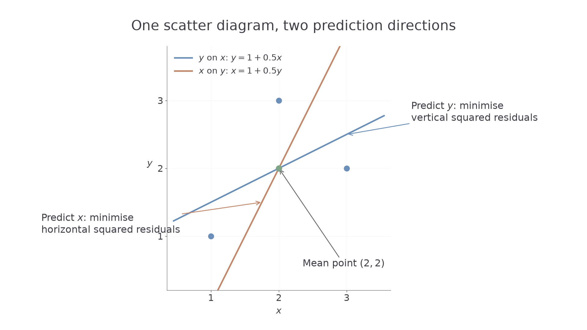
For the same three points, the two least squares lines meet at the mean point but give different predictions away from it

For non-constant variables, write the gradients in their native directions as $b_{yx} = S_{xy}/S_{xx}$ and $b_{xy} = S_{xy}/S_{yy}$ . Their product is

b_{yx}b_{xy} = \frac{S_{xy}^2}{S_{xx}S_{yy}} = r^2

This derived relationship is not in the formula booklet: learn it. It explains why the gradients are reciprocals only when $\lvert r\rvert = 1$ . When $r = 0$ , the lines are $y = \bar{y}$ and $x = \bar{x}$ : a horizontal line and a vertical line through the mean point.

Worked example 3: calculating both lines

Question. For observational paired data, neither variable is controlled. Given $\bar{x} = 10$ , $\bar{y} = 20$ , $S_{xx} = 40$ , $S_{yy} = 90$ and $S_{xy} = 48$ , calculate both regression lines.

Plan. Use the same numerator with the appropriate predictor's denominator, and write each line through the mean point.

\begin{aligned} b_{yx} &= \frac{48}{40} = \frac65 && x \text{ is the predictor} \\ y - 20 &= \frac65(x - 10) && \text{use the mean point} \\ y &= 8 + \frac65x && \text{expand} \\ b_{xy} &= \frac{48}{90} = \frac8{15} && y \text{ is the predictor} \\ x - 10 &= \frac8{15}(y - 20) && \text{use the same mean point} \\ x &= -\frac23 + \frac8{15}y && \text{expand} \end{aligned}

Why this step? Changing the response changes which residuals are minimised, so you must calculate the second gradient rather than invert the first.

Answer. For $y$ on $x$ , $y = 8 + \frac65x$ . For $x$ on $y$ , $x = -\frac23 + \frac8{15}y$ .

Check. Both contain $(10, 20)$ , and $\frac65 \times \frac8{15} = \frac{16}{25}$ , consistent with $r = 0.8$ .

Worked example 4 changes only the sign of $S_{xy}$ . The scatter now slopes downwards; both prediction coefficients change sign, but the mean point stays fixed.

Worked example 4: negative association

Question. Observational paired data have $\bar{x} = 10$ , $\bar{y} = 20$ , $S_{xx} = 40$ , $S_{yy} = 90$ and $S_{xy} = -48$ . Neither variable is controlled. Calculate both regression lines.

Plan. Calculate each negative coefficient and use the centred equations.

\begin{aligned} b_{yx} &= -\frac{48}{40} = -\frac65 && \text{predict } y \\ y - 20 &= -\frac65(x - 10) && \text{centre at the means} \\ y &= 32 - \frac65x && \text{expand} \\ b_{xy} &= -\frac{48}{90} = -\frac8{15} && \text{predict } x \\ x - 10 &= -\frac8{15}(y - 20) && \text{centre at the means} \\ x &= \frac{62}{3} - \frac8{15}y && \text{expand} \end{aligned}

Why this step? Negative correlation makes both native prediction gradients negative; it does not change which centred sum belongs underneath.

Answer. $y = 32 - \frac65x$ and $x = \frac{62}{3} - \frac8{15}y$ .

Check. At the mean point, $32 - 12 = 20$ and $\frac{62}{3} - \frac{32}{3} = 10$ . The gradient product is still $16/25$ , now corresponding to $r = -0.8$ .

Continue this lesson.

You’re previewing NovaLearn without an account. Create a free account to read the rest.

Create free account

Last Accessed

Pure Core

Statistics

Mechanics

Discrete Mathematics

Additional Pure Mathematics

5.09a–5.09e - Least squares regression lines

Variables and vertical residuals

Calculating the regression line

The two prediction directions

Continue this lesson.

Learn faster with Nova