5.03a–5.03d - Probability density, mean and variance | OCR A-Level Further Mathematics A

A continuous measurement assigns probability to intervals rather than individual values. In 5.03a–5.03b you will turn a density curve, including a piecewise curve, into probabilities; 5.03c–5.03d then use the same areas to find means, variances and expected values of functions.

Density and probability

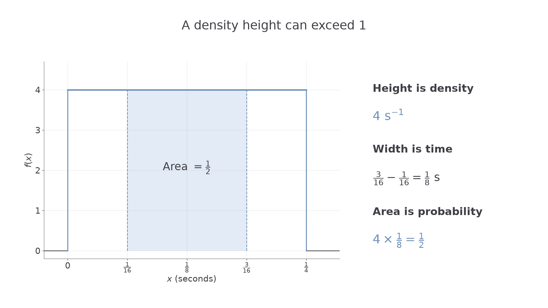
Can the height of a probability density curve be greater than $1$ , even though a probability cannot? Imagine a timer whose reading $X$ , in seconds, lies between $0$ and $\frac14$ , with equal probability in equal-length intervals. The rectangle under its density must have area $1$ , so its height is $4$ . A height of $4$ is perfectly sensible: a probability of $4$ is not.

You already know

For a discrete random variable, probabilities are attached to possible values and add to $1$ . A definite integral gives signed area; when the integrand is non-negative, it gives ordinary area. Expectation is a probability-weighted average.

Measurements such as a waiting time or a length are modelled on a continuous scale. The model may allow every value in an interval even when the measuring instrument rounds its display. A rounded reading of $2.0$ represents an interval, not the event that the underlying measurement is exactly $2$ .

[DIAGRAM: asset_name: Density height is not probability; asset_slug: h245_5_03_density_height; caption: A rectangle of height 4 and width one quarter has total area 1, while an interval of width one eighth has probability one half; description: Density graph on white axes with x in seconds. The density equals 4 from x equals 0 to x equals one quarter and zero elsewhere. A pale blue strip from one sixteenth to three sixteenths has width one eighth, height 4 and area one half. A side panel distinguishes density 4 per second from probability one half]
A rectangle of height 4 and width one quarter has total area 1, while an interval of width one eighth has probability one half

Continuous random variable and probability density

A continuous random variable $X$ has a probability density function $f$ when probabilities are given by areas:

\mathrm{P}(a<X<b)=\int_a^b f(x)\,dx

The density satisfies $f(x)\ge0$ for every $x$ , and its total area is $1$ . The support is the set of values on which the distribution is concentrated, usually described by the intervals where its density can be positive. For example, the timer has support $[0,\frac14]$ . A function with a negative section is not a valid p.d.f., even if its total signed integral is $1$ .

For a very short interval of width $h$ , the probability is approximately $f(x)h$ , provided the density varies little across the interval. Shrinking the interval to a single point leaves area zero. Thus $\mathrm{P}(X=c)=0$ , and including or excluding a single endpoint does not change any probability. This does not say that no value occurs: one value occurs on each trial, but no preselected exact value has positive probability.

A density carries reciprocal units: if $X$ is in seconds, $f(x)$ is in $\mathrm{s^{-1}}$ . Multiplying by a width in seconds gives a probability with no units. Altering a density at a finite number of individual points also leaves all probabilities unchanged.

Key idea

Density is height; probability is area. A continuous point has probability zero, while an interval can have positive probability.

The timer's density gives $\mathrm{P}(\frac1{16}<X<\frac3{16})=4(\frac3{16}-\frac1{16})=\frac12$ , exactly the shaded area. Use that distinction in the diagnostic question.

Validating a density

To determine an unknown constant in a density, make its total area equal to $1$ , then check non-negativity on the whole support.

Conditions for a p.d.f.

A valid probability density satisfies

f(x)\ge0\quad\text{for every }x, \qquad \int_{-\infty}^{\infty}f(x)\,dx=1

On finite or piecewise support, add the integrals over all the relevant intervals.
These conditions are not printed as a separate result in the booklet.
Not in the formula booklet: learn it.

Both conditions matter. A signed integral can equal $1$ even when the graph dips below the axis, and a non-negative curve can have the wrong total area. The first example keeps these two jobs separate.

Worked example 1: a normalising constant

Question. The function $f(x)=kx$ for $0\le x\le2$ , and $f(x)=0$ otherwise, is a probability density. Determine $k$ .

Plan. Integrate on the stated support, set the area equal to $1$ , and check the sign.

\begin{aligned} \int_0^2 kx\,dx&=1 &&\text{total probability}\\ \left[\frac{kx^2}{2}\right]_0^2&=1 &&\text{integrate}\\ 2k&=1 &&\text{insert limits}\\ k&=\frac12 &&\text{solve} \end{aligned}

Why this step? The limits come from the support; integrating over all real values adds only zero outside it.

Answer. $k=\frac12$ . Then $f(x)=\frac{x}{2}\ge0$ on $[0,2]$ , and it is zero elsewhere, so both conditions hold.

Check. The graph is a triangle of base $2$ and height $1$ , with area $\frac12\times2\times1=1$ .

Worked example 2 changes one feature: the density has two pieces. The constant must normalise their combined area, rather than making each piece have area $1$ .

Worked example 2: two pieces share one total

Question. Determine $k$ so that

f(x)=\begin{cases}kx&0\le x\le1\\k(2-x)&1<x\le2\\0&\text{otherwise}\end{cases}

is a valid probability density.

Plan. Add the two area integrals and check each piece is non-negative.

\begin{aligned} \int_0^1kx\,dx+\int_1^2k(2-x)\,dx&=1 &&\text{split at }1\\ \frac{k}{2}+\frac{k}{2}&=1 &&\text{evaluate both pieces}\\ k&=1 &&\text{solve} \end{aligned}

Why this step? There is one random variable and one unit of probability, shared between the two intervals.

Answer. $k=1$ . On the first interval $x\ge0$ ; on the second $2-x\ge0$ . The density is therefore non-negative everywhere, with total area $1$ .

Check. The two pieces form a triangle of base $2$ and height $1$ , again giving area $1$ . Each half has probability $\frac12$ .

The sign check is short, but it establishes something integration alone cannot establish.

Watch out

Wrong: “ $\int f(x)\,dx=1$ , so $f$ is a valid density.” An indefinite integral is not a total area, and area alone is insufficient. Right: use definite limits covering the support and also state $f(x)\ge0$ throughout.

In a “show that this is a valid p.d.f.” question, write both conditions explicitly. For a piecewise function, inspect every branch, including the zero branch.

Interval probabilities

An event chooses the area you need; the formula for the density tells you how to calculate it.

Probabilities from a density

For a continuous variable with p.d.f. $f$ ,

\mathrm{P}(a\le X\le b)=\int_a^b f(x)\,dx

The same value applies with either or both inequalities strict. Restrict the integral to the support, and split it wherever the expression for $f$ changes.
The booklet gives the c.d.f. integral, from which this result follows, but does not print this interval rule separately.
Not in the formula booklet: learn it.

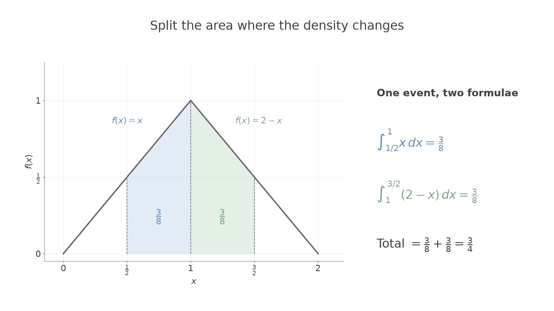
The two-piece density from the preceding example has $k=1$ . Its area from $0$ to $1$ is $\frac12$ ; its area from $1$ to $2$ is the remaining $\frac12$ . An interval crossing $1$ needs both expressions.

[DIAGRAM: asset_name: Split a probability at the density join; asset_slug: h245_5_03_piecewise_area; caption: The interval from one half to three halves crosses the join at 1, so its probability is the sum of two shaded integrals; description: Triangular density f(x) equals x on 0 to 1 and 2 minus x on 1 to 2, with zero density elsewhere. Blue shading covers one half to 1 and sage shading covers 1 to three halves. Each shaded area is three eighths and their total is three quarters. The two integrals are written in a separate side panel]
The interval from one half to three halves crosses the join at 1, so its probability is the sum of two shaded integrals

Worked example 3: an interval within one piece

Question. Let $f(x)=x$ for $0\le x\le1$ , $f(x)=2-x$ for $1<x\le2$ , and zero otherwise. Find $\mathrm{P}(\frac14<X<\frac34)$ .

Plan. Both limits lie in the first piece, so integrate $x$ between them.

\begin{aligned} \mathrm{P}\left(\frac14<X<\frac34\right)&=\int_{1/4}^{3/4}x\,dx &&\text{choose the first branch}\\ &=\left[\frac{x^2}{2}\right]_{1/4}^{3/4} &&\text{integrate}\\ &=\frac9{32}-\frac1{32}=\frac14 &&\text{subtract endpoint values} \end{aligned}

Why this step? The density formula outside this event contributes no area to this probability.

Answer. $\frac14$ .

Check. The region is a trapezium with parallel sides $\frac14$ and $\frac34$ , separated by $\frac12$ , so its area is $\frac12(\frac14+\frac34)\frac12=\frac14$ .

Worked example 4 changes only the interval: it now crosses the join. Keeping one expression throughout would give the wrong area.

Continue this lesson.

You’re previewing NovaLearn without an account. Create a free account to read the rest.

Create free account

Last Accessed

Pure Core

Statistics

Mechanics

Discrete Mathematics

Additional Pure Mathematics

5.03a–5.03d - Probability density, mean and variance

Density and probability

Validating a density

Interval probabilities

Continue this lesson.

Learn faster with Nova