7.08e, 7.08f - Optimal mixed strategies | OCR A-Level Further Mathematics A

Use random choices to improve a player's guaranteed expected pay-off when a game has no stable pure solution. You will solve two-choice games with equations and graphs, include endpoint probabilities and formulate larger games as linear programmes that can be solved by simplex.

Mixed strategies and indifference

In a game with A pay-off matrix $\begin{pmatrix}4 & 0 \\ 0 & 3\end{pmatrix}$ , either pure choice lets B hold A to zero: can an unpredictable choice guarantee A a positive expected pay-off? The answer depends on choosing the probabilities, rather than taking turns in a pattern B can exploit.

You already know

In an A pay-off matrix, A maximises and B minimises. A's play-safe pure value is the largest row minimum; B's is the smallest column maximum. Expected value is found by multiplying each outcome by its probability and adding.

A should choose privately and randomly on each play. “Use P three times, then Q four times” gives the same long-run proportions as some random strategy, but its predictable order could reveal the next choice. An expected guarantee concerns average pay-off over repeated plays, not a lower bound on every individual result.

Mixed strategy

A mixed strategy specifies the probabilities with which a player randomly chooses their available pure strategies. The probabilities are non-negative and sum to $1$ . For two choices, write the probabilities as $p$ and $1 - p$ , where $0 \le p \le 1$ . The endpoints are pure strategies, included when finding the optimum.

If A randomises between two rows, calculate the expected pay-off separately against each fixed column. B can select the smallest of those expectations, so A maximises their minimum. A mixture of columns cannot reduce the expectation below the smallest individual column expectation.

Expected pay-off against a fixed choice

If A plays rows P and Q with probabilities $p$ and $1 - p$ , and a fixed column gives pay-offs $a$ and $b$ , then

E = ap + b(1 - p),\qquad 0 \le p \le 1

A maximises the minimum of the column expectations. If B randomises between two columns, B minimises the maximum of the row expectations, when they are still measured as A's pay-offs.

Not in the formula booklet: learn it.

An interior optimum often makes the opponent indifferent between two active choices. Equating their expectations finds a candidate; checking the remaining choices and endpoints establishes that it is optimal.

Worked example 1: improving on both pure guarantees

Question. For the following A pay-off matrix, determine the optimal mixed strategies for both players and the value of the game to A.

\begin{array}{c|rr} & \mathrm{X} & \mathrm{Y} \\ \hline \mathrm{P} & 4 & 0 \\ \mathrm{Q} & 0 & 3 \end{array}

Plan. Make B's two columns equally attractive when A mixes, then make A's two rows equally attractive when B mixes.

Let A play P with probability $p$ and Q with probability $1 - p$ .

\begin{aligned} E_{\mathrm{X}} &= 4p && \text{B chooses X} \\ E_{\mathrm{Y}} &= 3(1 - p) && \text{B chooses Y} \\ 4p &= 3 - 3p && \text{equate the two bounds} \\ p &= \frac{3}{7},\qquad v = \frac{12}{7} && \text{solve and substitute} \end{aligned}

Below $p = 3/7$ , the smaller expression $4p$ increases; above it, the smaller expression $3 - 3p$ decreases. Thus this intersection maximises the minimum.

Let B play X with probability $q$ and Y with probability $1 - q$ .

\begin{aligned} E_{\mathrm{P}} &= 4q,\qquad E_{\mathrm{Q}} = 3(1 - q) && \text{A's row expectations} \\ 4q &= 3 - 3q && \text{make A indifferent} \\ q &= \frac{3}{7} && \text{minimise A's maximum} \end{aligned}

Why this step? A's mixture guarantees at least $12/7$ , while B's mixture holds A to at most $12/7$ . The matching bounds prove optimality for both.

Answer. A plays P, Q with probabilities $3/7$ , $4/7$ . B plays X, Y with probabilities $3/7$ , $4/7$ . The value to A is $12/7$ , and the value to B is $-12/7$ .

Check. Both endpoint choices for A guarantee $0$ , less than $12/7$ . Each probability pair sums to $1$ , and all probabilities lie between $0$ and $1$ .

The second example changes only the Q, Y pay-off, from $3$ to $2$ . The less rewarding Q outcome changes the balance of probabilities.

Worked example 2: changing one reward

Question. Determine both optimal mixed strategies and the value to A for

\begin{array}{c|rr} & \mathrm{X} & \mathrm{Y} \\ \hline \mathrm{P} & 4 & 0 \\ \mathrm{Q} & 0 & 2 \end{array}

Plan. Equate the expected pay-offs against X and Y for A, then against P and Q for B.

\begin{aligned} E_{\mathrm{X}} &= 4p,\qquad E_{\mathrm{Y}} = 2 - 2p && \text{A mixes between rows} \\ 4p &= 2 - 2p && \text{intersection of the bounds} \\ p &= \frac{1}{3},\qquad v = \frac{4}{3} && \text{solve for A} \end{aligned}

The minimum increases towards this intersection from the left and decreases after it. For B,

\begin{aligned} E_{\mathrm{P}} &= 4q,\qquad E_{\mathrm{Q}} = 2 - 2q && \text{expectations still for A} \\ 4q &= 2 - 2q && \text{equate A's two choices} \\ q &= \frac{1}{3} && \text{solve for B} \end{aligned}

Why this step? B minimises A's best expected outcome. Keeping all expectations in A's units avoids an unnecessary sign change during the calculation.

Answer. A plays P, Q with probabilities $1/3$ , $2/3$ ; B plays X, Y with probabilities $1/3$ , $2/3$ . The value to A is $4/3$ .

Check. Against A's mixture, X gives $4(1/3) = 4/3$ , and Y gives $2(2/3) = 4/3$ . Against B's mixture, either row gives that same value.

The probabilities for A and B happen to be equal in these diagonal matrices. That is a feature of these games, not a general rule: solve separately for each player's mixture.

Watch out

Wrong: “A's probability tells B how often to choose X.” A's probabilities describe rows; B's describe columns. They come from different expected-pay-off equations, even when the answers happen to match.

Balance the two active expectations in a new game.

The lower envelope for the row player

With two rows and several columns, A still needs only one probability $p$ . Each column supplies a straight line, and B can choose whichever line is lowest at that $p$ .

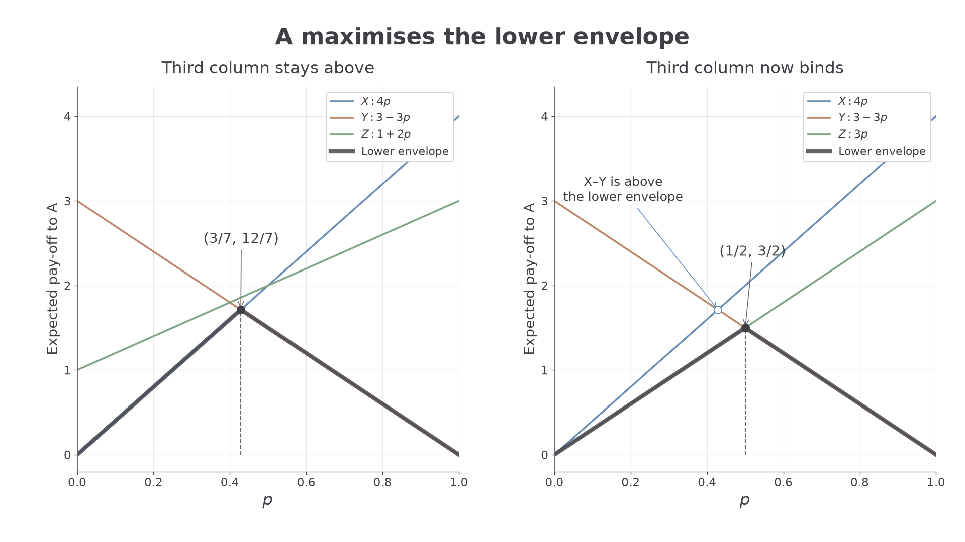
The curve made from the lowest pieces is the lower envelope. A wants its highest point. An intersection above the envelope is irrelevant to the guarantee, because another column then gives A less.

Lower-envelope optimum

For a two-row A pay-off matrix, plot each column's expected pay-off against $p$ , the probability of the first row, over $0 \le p \le 1$ . The optimal choice for A maximises the lower envelope, the minimum of all plotted expectations. Check the relevant intersections and both endpoints.

The graphical rule is not printed in the formula booklet. Learn which envelope belongs to the player whose pay-off the matrix records, rather than memorising an unlabelled picture.

[DIAGRAM: asset_name: Selecting the highest point of the lower envelope; asset_slug: h245_7_08_lower_envelopes; caption: A maximises the lowest available expectation, so changing one third-column entry changes which intersection is relevant; description: Two graphs have horizontal probability axis p from 0 to 1. Left graph plots X equal 4p, Y equal 3 minus 3p and Z equal 1 plus 2p; the thick lower envelope has highest point at p equal 3 sevenths, E equal 12 sevenths, where X and Y meet below Z. Right graph changes Z to 3p; the thick lower envelope now peaks at p equal one half, E equal three halves, where Y and Z meet. The X Y intersection is marked as above the lower envelope. Each graph has labelled scales and a legend]
A maximises the lowest available expectation, so changing one third-column entry changes which intersection is relevant

Worked example 3: a third column that does not bind

Question. Use a graphical method to determine A's optimal mixed strategy and the value of this game to A.

\begin{array}{c|rrr} & \mathrm{X} & \mathrm{Y} & \mathrm{Z} \\ \hline \mathrm{P} & 4 & 0 & 3 \\ \mathrm{Q} & 0 & 3 & 1 \end{array}

Plan. Form the three expected-pay-off lines and locate the highest point of their lower envelope.

For A's probability $p$ of P,

\begin{aligned} E_{\mathrm{X}} &= 4p && \text{first column} \\ E_{\mathrm{Y}} &= 3 - 3p && \text{second column} \\ E_{\mathrm{Z}} &= 1 + 2p && \text{third column} \end{aligned}

The left-hand graph shows X and Y meeting on the lower envelope.

\begin{aligned} 4p &= 3 - 3p && \text{intersection on the envelope} \\ p &= \frac{3}{7},\qquad E_{\mathrm{X}} = E_{\mathrm{Y}} = \frac{12}{7} && \text{solve} \\ E_{\mathrm{Z}} &= 1 + \frac{6}{7} = \frac{13}{7} > \frac{12}{7} && \text{third column does not lower it} \end{aligned}

Why this step? The third line must be checked at the proposed optimum. Equating two expressions without checking the others may overstate the guarantee.

Answer. A plays P with probability $3/7$ and Q with probability $4/7$ . The lower envelope rises to $12/7$ and then falls, so the value to A is $12/7$ .

Check. At $p = 0$ and $p = 1$ , the lower envelope is $0$ . Also, B can mix X and Y with probabilities $3/7$ , $4/7$ , holding either A row to $12/7$ .

The next example changes only the Q, Z entry, from $1$ to $0$ . The former X, Y intersection will no longer lie on the lower envelope.

Worked example 4: rejecting an irrelevant intersection

Question. Use a graphical method to determine A's optimal mixed strategy for

\begin{array}{c|rrr} & \mathrm{X} & \mathrm{Y} & \mathrm{Z} \\ \hline \mathrm{P} & 4 & 0 & 3 \\ \mathrm{Q} & 0 & 3 & 0 \end{array}

and find the value to A.

Plan. Replace the changed line, then use the intersection that actually bounds the minimum expectation.

\begin{aligned} E_{\mathrm{X}} &= 4p,\quad E_{\mathrm{Y}} = 3 - 3p,\quad E_{\mathrm{Z}} = 3p && \text{three column expectations} \\ 3p &\le 4p && \text{Z is no higher than X on }[0, 1] \\ 3p &= 3 - 3p && \text{active lines Z and Y} \\ p &= \frac{1}{2},\qquad v = \frac{3}{2} && \text{highest lower-envelope point} \end{aligned}

Why this step? At the X, Y intersection $p = 3/7$ , Z gives only $9/7$ . The apparent height $12/7$ is therefore not guaranteed.

Answer. A uses P and Q equally, with probabilities $1/2$ , $1/2$ . The value to A is $3/2$ .

Check. At $p = 1/2$ , the three expectations are $2$ , $3/2$ , $3/2$ . Before this point the lower line $3p$ increases; afterwards $3 - 3p$ decreases. Both endpoints give $0$ .

The graph explains the choice of equations. In an exam, show labelled axes spanning $0$ to $1$ , the relevant lines and the chosen intersection, even if a calculator helps you locate it.

Watch out

Wrong: “Choose the highest intersection.” An intersection can sit above a third line, leaving B a cheaper response. Right: choose the highest point of the lower envelope and verify every other expectation there.

Identify the binding columns before solving the next pair of equations.

The upper envelope and endpoint solutions

If B has two columns, use a probability for B's first column and calculate A's expected pay-off separately for each row. A can choose the largest, so B wants the lowest point of the upper envelope.

There is no need to transpose or negate the matrix if you keep stating that the vertical axis measures A's pay-off. If instead you negate and transpose to make B the row player with B's pay-offs, you may use a lower envelope; the signs and player labels must change together.

Upper-envelope optimum

For a two-column A pay-off matrix, plot each row's expected pay-off against $p$ , B's probability of choosing the first column. B minimises the upper envelope, the maximum of the row expectations, over $0 \le p \le 1$ . The optimum can be at an intersection or at $p = 0$ or $p = 1$ . An endpoint gives a pure choice rather than a genuine mixture.

This graphical rule and the need to check endpoint probabilities are not printed in the formula booklet. A graph can reveal a stable pure solution, even when you initially set up the calculation expecting to mix.

Continue this lesson.

You’re previewing NovaLearn without an account. Create a free account to read the rest.

Create free account

Last Accessed

Pure Core

Statistics

Mechanics

Discrete Mathematics

Additional Pure Mathematics

7.08e, 7.08f - Optimal mixed strategies

Mixed strategies and indifference

The lower envelope for the row player

The upper envelope and endpoint solutions

Continue this lesson.

Learn faster with Nova