5.05c - Hypothesis tests for a population mean | OCR A-Level Further Mathematics A

Use a normal distribution to decide whether sample data provide significant evidence about a population mean. You will choose the correct tail, distinguish a known population variance from an estimated one, and write a conclusion that says what the evidence supports without claiming certainty.

Hypotheses and the sampling model

A measuring process is meant to have population mean $50$ . A sample mean is $51.8$ . Is that evidence of a shift, or an ordinary fluctuation? The gap alone cannot answer: you need the spread of sample means and the direction of the claim.

A hypothesis test temporarily assumes a stated population mean. It asks whether a sample result at least as extreme as yours would be unusual under that assumption. It does not calculate the probability that the assumption is true.

You already know

For a random independent sample, $\mathrm{E}(\overline X)=\mu$ and $\mathrm{Var}(\overline X)=\sigma^2/n$ . A normal population makes $\overline X$ exactly normal; a sufficiently large sample from another population with finite variance makes its distribution approximately normal. Estimate an unknown variance using $s^2$ , with denominator $n-1$ .

Write hypotheses about the population parameter, not the observed sample mean. Define the parameter in context before using its symbol.

Null and alternative hypotheses

The null hypothesis $\mathrm{H}_0$ specifies the population mean $\mu=\mu_0$ . The alternative $\mathrm{H}_1$ is the claim being tested: $\mu>\mu_0$ , $\mu<\mu_0$ , or $\mu\ne\mu_0$ . An increase or decrease gives a one-tailed test; a difference in either direction gives a two-tailed test.

For example, if $\mu$ is the population mean output of a measuring process, “has increased from $50$ ” gives $\mathrm{H}_0:\mu=50$ , $\mathrm{H}_1:\mu>50$ . “Has changed from $50$ ” gives $\mathrm{H}_1:\mu\ne50$ . Choose the alternative from the question before inspecting the sample result.

Population and sample	Distribution used for the mean under $\mathrm{H}_0$	Reason
Normal population, known, given or assumed variance $\sigma^2$ ; any sample size	$\mathrm{N}(\mu_0,\sigma^2/n)$ , exactly	Independent normal observations
Any population with finite known, given or assumed variance $\sigma^2$ ; large sample	$\mathrm{N}(\mu_0,\sigma^2/n)$ , approximately	Central limit theorem
Any population with finite unknown variance; large sample	$\mathrm{N}(\mu_0,s^2/n)$ , approximately	Central limit theorem and estimated variance

All three cases require random independent observations from the population being tested. A small sample from an unspecified population does not justify a normal test. A normal population with unknown variance and a small sample is also outside these normal-test cases.

p-value and significance level

A p-value is the probability, assuming $\mathrm{H}_0$ and the model, of a test result at least as extreme as the observed one in the direction or directions specified by $\mathrm{H}_1$ . The significance level $\alpha$ is the preselected threshold for rejecting $\mathrm{H}_0$ .

For a continuous normal test, reject $\mathrm{H}_0$ when the p-value is at most $\alpha$ ; otherwise do not reject it. This decision rule is not printed in the formula booklet: learn it. Under a correct exact null model, a $5\%$ test still rejects a true null in $5\%$ of repetitions. A rare result is evidence, not a logical contradiction.

Key idea

Build the sampling distribution around the null mean $\mu_0$ , then locate the observed sample mean $\overline x$ within it. The data provide the observation; they do not replace the null mean at the centre.

The first decision is linguistic as well as mathematical: decide which population claim the question is asking you to examine.

One-tailed tests with known variance

For a known normal population variance, standardise the sample mean using its standard error. Keep the sign: it tells you which side of the null mean the observation occupies.

Standardising under a normal null model

If the population is normal with known, given or assumed variance $\sigma^2$ , then under $\mathrm{H}_0:\mu=\mu_0$ ,

Z=\frac{\overline X-\mu_0}{\sigma/\sqrt n}\sim\mathrm{N}(0,1)

The observed value is $z=(\overline x-\mu_0)/(\sigma/\sqrt n)$ . Random independent sampling is required.

In the formula booklet.

For an upper-tail alternative use $\mathrm{P}(Z\ge z)$ ; for a lower-tail alternative use $\mathrm{P}(Z\le z)$ . These tail-selection rules are not printed in the formula booklet: learn them. Equivalently, at the $5\%$ level the upper critical value is $1.64485\ldots$ and the lower critical value is $-1.64485\ldots$ ; normal percentage points are supplied in the booklet. Do not choose a small tail merely because it gives a significant result.

Worked example 1: evidence of an increase

Question. A measuring process has normally distributed outputs with known variance $16$ . A random independent sample of $16$ outputs has mean $51.8$ . Test, at the $5\%$ significance level, whether its population mean has increased from $50$ .

Plan. Define the population mean, use the null sampling distribution, and compare its upper-tail probability with $0.05$ .

Let $\mu$ be the population mean output. Then $\mathrm{H}_0:\mu=50$ , $\mathrm{H}_1:\mu>50$ .

\begin{aligned} \overline X&\sim\mathrm{N}(50,16/16) &&\text{under }\mathrm{H}_0\\ z&=\frac{51.8-50}{4/\sqrt{16}}=1.8 &&\text{standard error }1\\ p&=\mathrm{P}(Z\ge1.8)=0.035930\ldots &&\text{upper tail}\\ p&<0.05 &&\text{significance comparison} \end{aligned}

Why this step? The population standard deviation is $4$ , but the random quantity being tested is an average of $16$ outputs, whose standard deviation is $1$ .

Answer. Reject $\mathrm{H}_0$ . There is sufficient evidence at the $5\%$ level that the population mean output has increased from $50$ .

Check. The critical sample mean is $50+1.64485\ldots(1)=51.64485\ldots$ . The observed mean $51.8$ lies above it.

Worked example 2 changes only the observed sample mean. The same method now illustrates what a non-significant result allows you to say.

Worked example 2: an increase too small to establish

Question. The same normal process, with known variance $16$ , gives a random independent sample of $16$ outputs with mean $51.2$ . Test, at the $5\%$ level, whether its population mean has increased from $50$ .

Plan. Use the same hypotheses and null standard error, with the new observation.

Let $\mu$ be the population mean output, with $\mathrm{H}_0:\mu=50$ , $\mathrm{H}_1:\mu>50$ .

\begin{aligned} z&=\frac{51.2-50}{4/\sqrt{16}}=1.2 &&\text{new sample mean}\\ p&=\mathrm{P}(Z\ge1.2)=0.115069\ldots &&\text{upper tail}\\ p&>0.05 &&\text{not significant} \end{aligned}

Why this step? A sample mean above $50$ is not enough by itself. The upper-tail probability measures how surprising this increase is under $\mathrm{H}_0$ .

Answer. Do not reject $\mathrm{H}_0$ . There is insufficient evidence at the $5\%$ level that the population mean output has increased from $50$ .

Check. $51.2<51.64485\ldots$ , so the observed sample mean is outside the upper critical region.

If the claim had instead been a decrease, these positive test statistics would give large lower-tail probabilities. Data in the opposite direction do not support a one-tailed claim.

Watch out

Wrong: “Do not reject $\mathrm{H}_0$ , so the population mean is $50$ .” A non-significant result does not establish equality. Right: “There is insufficient evidence that the population mean has increased from $50$ .” Keep the conclusion in context and at the stated level.

Now change the direction of the claim. The hypotheses are supplied so you can concentrate on the lower tail.

Two-tailed tests and large samples

A claim that a population mean has changed must allow evidence in either direction. At the $5\%$ significance level, each normal tail receives $2.5\%$ , not $5\%$ .

[DIAGRAM: asset_name: One-tailed and two-tailed critical regions; asset_slug: h245_5_05_critical_tails; caption: A 5 percent upper-tail test uses 1.645 while a 5 percent two-tail test uses minus and plus 1.960; description: Two standard normal density plots. The left plot shades the upper 0.05 tail beyond 1.645. The right plot shades each 0.025 tail beyond minus 1.960 and plus 1.960, with observed z equal to 1.8 marked to show it is significant only for the upper-tail alternative.]
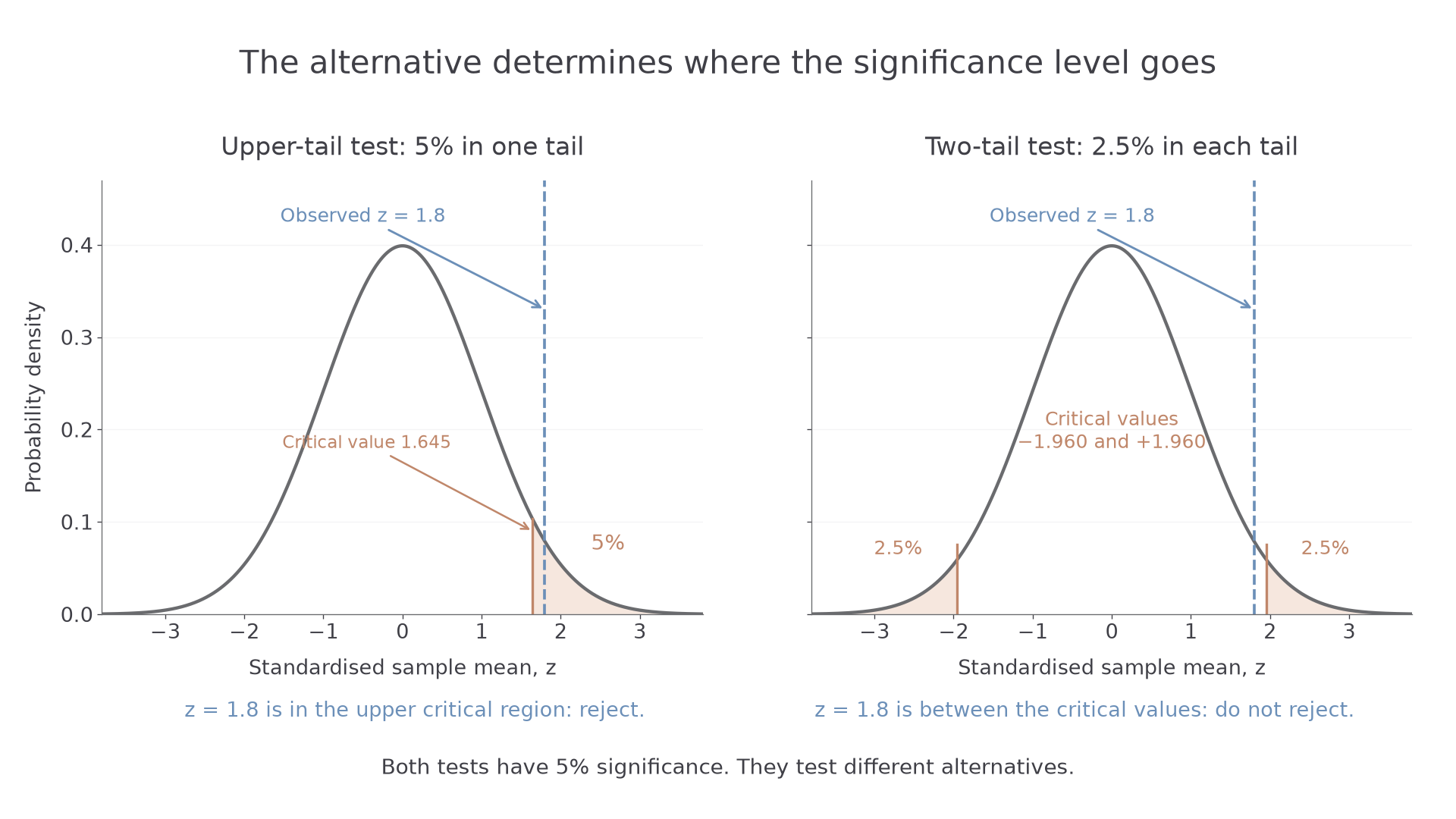
A 5 percent upper-tail test uses 1.645 while a 5 percent two-tail test uses minus and plus 1.960

For a large independent sample from an unspecified population, use the central limit theorem for the shape of $\overline X$ . Its mean and variance still come from the exact sampling-moment formulae. If the population variance is known, do not introduce an estimated-variance correction.

A two-tailed normal mean test

For a normal or approximately normal sample mean under $\mathrm{H}_0$ , with known variance $\sigma^2$ , calculate

z=\frac{\overline x-\mu_0}{\sigma/\sqrt n}, \qquad p=2\mathrm{P}(Z\ge|z|),\quad Z\sim\mathrm{N}(0,1)

Reject at level $\alpha$ if $p\le\alpha$ . Equivalently, reject if $|z|\ge z_{1-\alpha/2}$ , where $\mathrm{P}(Z\le z_{1-\alpha/2})=1-\alpha/2$ . The standardisation and normal percentage points are supplied, but this two-tailed decision rule is not printed.

Not in the formula booklet: learn it.

Continue this lesson.

You’re previewing NovaLearn without an account. Create a free account to read the rest.

Create free account

Last Accessed

Pure Core

Statistics

Mechanics

Discrete Mathematics

Additional Pure Mathematics

5.05c - Hypothesis tests for a population mean

Hypotheses and the sampling model

One-tailed tests with known variance

Two-tailed tests and large samples

Continue this lesson.

Learn faster with Nova