5.07f - Normal approximations for Wilcoxon tests

Which rank sum is approximately normal?

With $30$ signed ranks, the positive ranks sum to $330$. Is that unusually large, or simply a large number because there are many ranks? The total available is $1+\cdots+30=465$; under the null, the expected positive share is half, $232.5$. You need its spread before judging the evidence.

For signed ranks, under a continuous symmetric null population, each rank is equally likely to receive a positive or negative sign. The positive sum is therefore a sum of independent contributions: rank $r$ contributes either $0$ or $r$, each with probability $1/2$. Many contributions produce a roughly bell-shaped distribution. The normal approximation concerns $W^+$ or $W^-$ separately.

The minimum $T=\min(W^+,W^-)$ cannot exceed half the total. Its distribution is folded and is not the normal distribution printed in the booklet. Similarly, for independent samples the normal approximation applies to the raw rank sum $R_m$, not to the folded small-sample-table statistic $W$.

The large-sample approximation keeps the original sampling assumptions. Signed-rank observations, or paired differences, must be independent and continuous with a symmetric population distribution. For rank-sum tests, the two random samples must be independent, with identical continuous population distributions under the null. There are no zero signed differences or tied ranks in the calculations here.

Use the signed-rank approximation for sufficiently large $n$; the supplied exact table runs to $n=20$. For the rank-sum approximation both sample sizes must be sufficiently large. One large group does not by itself justify approximating a tiny group's rank-sum distribution. There is no single universal sample-size cut-off that replaces checking the model and the question's stated conditions.

The error below occurs before any standardisation. A correct variance cannot repair the wrong random variable.

A normal approximation for signed ranks

Use the observed positive rank sum and choose its tail from the median alternative. An integer sum includes a whole unit-wide interval in the continuous approximation.

Under the null, rank $r$'s mean contribution is $r/2$ and its variance is $r^2/4$. Adding these contributions explains the supplied mean and variance: half the rank total is the mean, and a quarter of the sum of squared ranks is the variance.

The continuity correction follows the event. For an integer statistic $S$, the event $S\ge s$ becomes $Y>s-0.5$; $S\le s$ becomes $Y<s+0.5$, where $Y$ is the continuous approximation. Strict inequalities first become their equivalent inclusive integer events: $S>s$ means $S\ge s+1$, hence boundary $s+0.5$. This event rule is not printed in the booklet: learn it.

[DIAGRAM: asset_name: A rank sum includes its whole unit interval; asset_slug: h245_5_07_continuity_correction; caption: An upper-tail event from 330 starts at 329.5 in the normal approximation; description: A normal curve with mean 232.5 and standard deviation about 48.62 has the area to the right of 329.5 shaded blue. An enlarged integer strip below shows blocks for rank sums 328 through 332, with the block centred at 330 spanning 329.5 to 330.5 and a vertical dashed boundary at 329.5.]

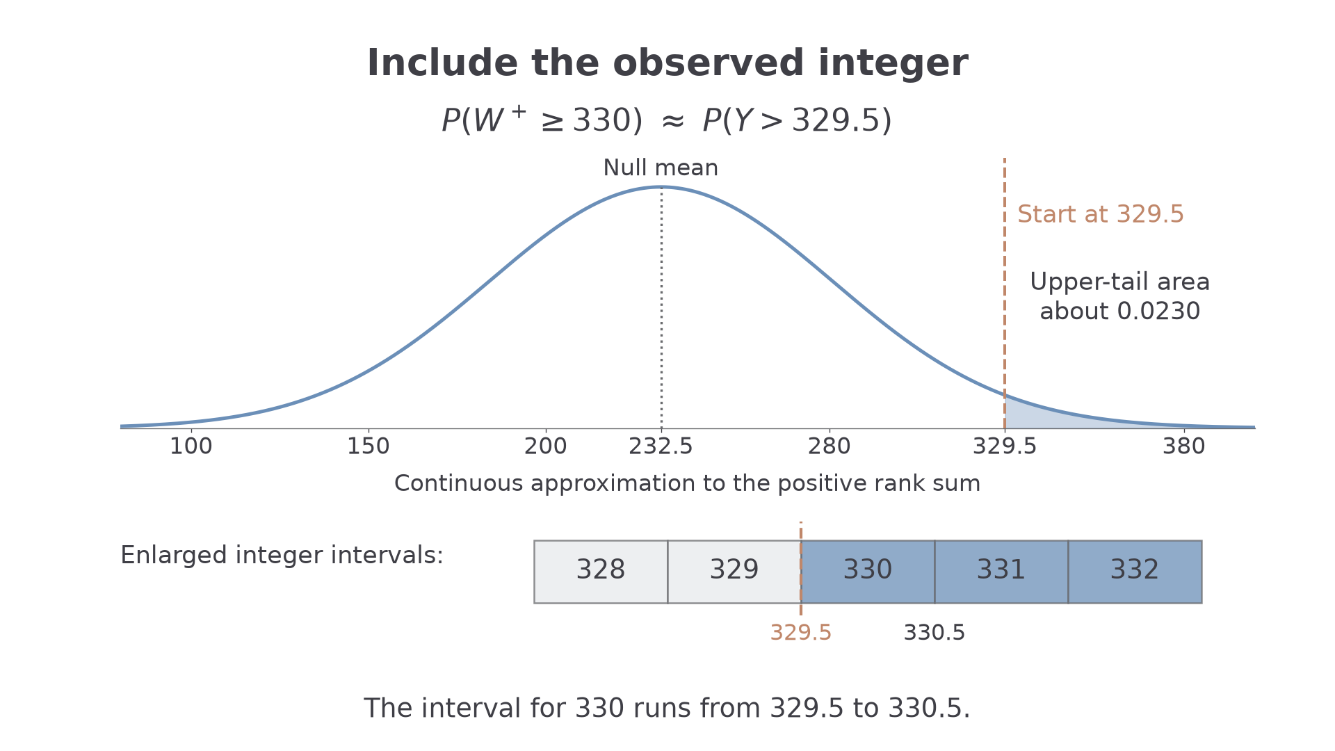
The boundary lies half a unit before the first included integer. It is chosen from the event, not from whether the observed sum happens to lie above or below its mean.

Worked example 2 reflects the evidence: the alternative is now a smaller median and the positive rank sum is $135$. The corrected lower tail should give the same probability.

Both examples answer the opening question: $330$ is roughly two null standard deviations above the expected positive sum, with one-sided approximate probability $0.0230$.

Use the same event-first reasoning with a different sample size and supplied hypotheses.

A normal approximation for independent rank sums

For two independent groups, approximate the raw sum of the smaller sample's pooled ranks. There is no subtraction of paired measurements and no signed-rank sample size.

Let the sample sizes be $m\le n$. Under identical continuous population distributions, each of the $m$ observations has expected pooled rank $(m+n+1)/2$. Multiplying by $m$ gives the null rank-sum mean. The ranks are sampled without replacement, so the supplied variance accounts for their dependence; treating the ranks as independent uniform draws would give a different variance.