5.02d, 5.02e - Binomial and discrete uniform models

Binomial means and variances

Two games can have the same average score but quite different uncertainty. How can you tell their spreads apart without constructing every probability? For standard distributions, their parameters give the mean and variance directly.

Each trial contributes an average of $p$ successes. Across $n$ trials, $np$ is the average total. The variance also depends on the chance of failure: if success is certain, the count is constant and has no spread. The following results may be used without proof.

When $0<p<1$, the variance is smaller than the mean. This is a property of the distribution, not a requirement that a finite sample's calculated moments satisfy an exact identity.

Change only what is known: the moments are supplied instead of the parameters. Dividing the two equations removes $n$.

An algebraic solution for $n$ must pass the integer check. Exact proposed moments giving a non-integer $n$ cannot belong to a binomial distribution, although rounded sample summaries need more cautious interpretation.

Reverse the calculation with new moments.

Equally likely integers

A discrete uniform distribution is appropriate when every integer in a specified consecutive list is equally likely. The word uniform describes the probabilities, not the spacing alone: an ordinary loaded die still has consecutive integer labels.

The notation is specific: $\mathrm{U}(8)$ means $1$ to $8$, not $0$ to $8$, and not every real value between the endpoints. Selecting uniformly from a larger consecutive integer list can be handled by coding a variable of this form.

[DIAGRAM: asset_name: Discrete uniform probability masses; asset_slug: h245_5_02_uniform_masses; caption: U(8) has eight probability masses of height 1/8, with no probability between the integers. The masses for X greater than 6 are highlighted; description: A probability-mass plot on white axes has points and stems at integers 1 through 8, all of height 0.125. The stems at 7 and 8 are clay, the others blue. Text identifies two qualifying values out of eight and distinguishes point probabilities from a continuous area]

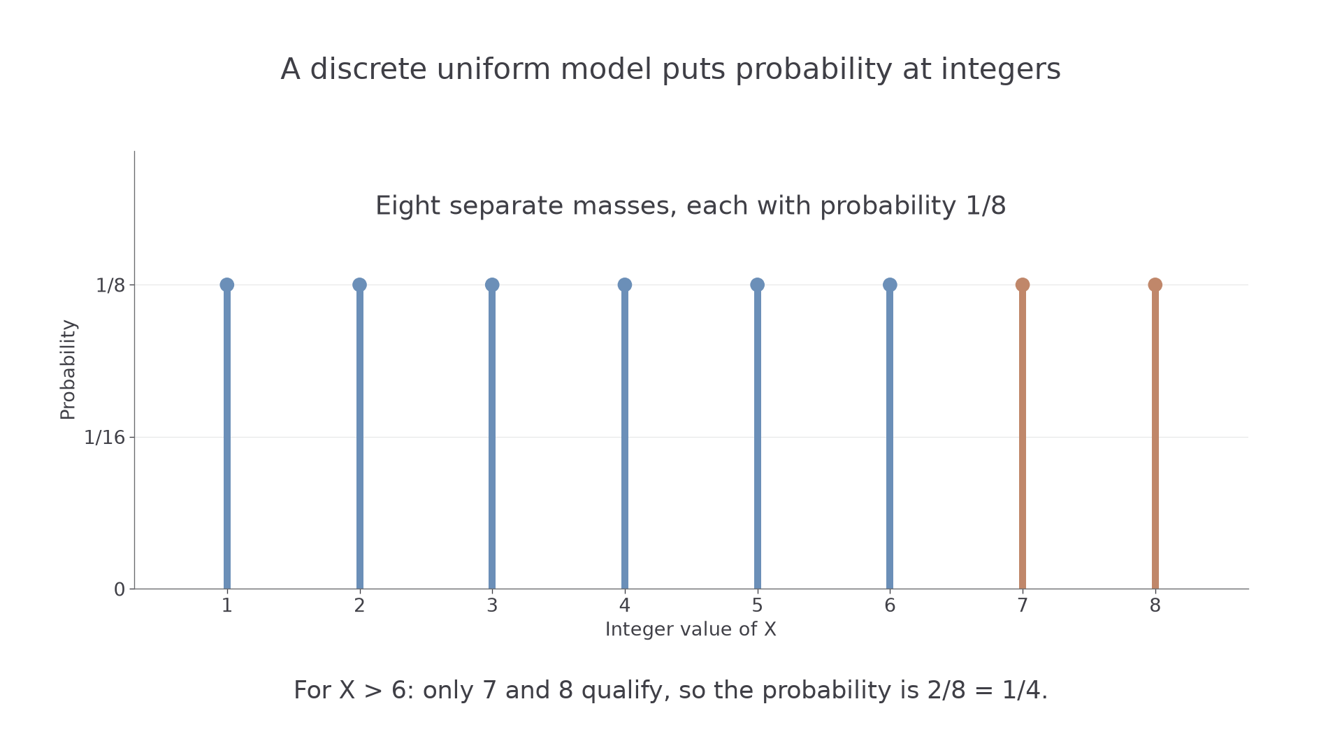
For any event involving a subset of those integers, count the qualifying values and divide by $n$. This follows by adding their equal probabilities; it is not a separate formula in the booklet. The individual probability $1/n$ is provided in its discrete-distributions table.