5.03a - Continuous uniform and exponential distributions | OCR A-Level Further Mathematics A

A constant density models equal chances across equal-length intervals; an exponential density models waiting for events arriving at a constant rate. This lesson develops the named continuous distributions in 5.03a, recalls how the normal model fits alongside them, and connects exponential waiting times to Poisson counts.

The continuous uniform model

If you have already waited $20$ minutes for an event, should your chance of waiting another $20$ minutes change? The answer depends on the model. We will compare a waiting time with a fixed upper limit against a waiting time with no fixed deadline, and return to this question at the end.

You already know

For a continuous variable, probabilities are areas, and $F(x)=\mathrm{P}(X\le x)$ . The normal model $X\sim\mathrm{N}(\mu,\sigma^2)$ from A-level Mathematics has a symmetric, bell-shaped density on the whole real line, with mean $\mu$ and variance $\sigma^2$ . Its p.d.f., mean and variance are in the formula booklet; calculate its probabilities by the normal tools you already know.

Suppose a timer stops at a time equally likely to lie anywhere between $2$ and $8$ seconds. An interval of length $1$ second has probability $\frac16$ , wherever it lies within that range. The density is a rectangle: width $6$ , height $\frac16$ , total area $1$ .

Continuous uniform distribution

A continuous uniform distribution over $[a,b]$ , with $a<b$ , has equal probabilities for equal-length intervals within that support. Its density is constant on $[a,b]$ and zero elsewhere. Not an example: equal probabilities at individual points, which all have probability zero for every continuous model.

The continuous model is different from the discrete uniform distribution $U(n)$ over the integers $1,2,\ldots,n$ . State the interval explicitly when using the continuous model.

Continuous uniform density and moments

For a continuous uniform variable on $[a,b]$ , where $a<b$ ,

f(x)=\begin{cases}\dfrac1{b-a}&a\le x\le b\\0&\text{otherwise}\end{cases}

\mathrm{E}(X)=\frac{a+b}{2},\qquad \mathrm{Var}(X)=\frac{(b-a)^2}{12}

In the formula booklet.

The mean is the midpoint by symmetry. You can recover the variance by integrating about that midpoint: writing $L=b-a$ ,

\frac1L\int_{-L/2}^{L/2}u^2\,du=\frac{L^2}{12}

The c.d.f. increases linearly from $0$ to $1$ : it is $0$ below $a$ , $\frac{x-a}{b-a}$ on $[a,b]$ , and $1$ above $b$ . This c.d.f. is not printed in the booklet: learn how to obtain it from the rectangular area.

[DIAGRAM: asset_name: A continuous uniform density; asset_slug: h245_5_03_uniform_density; caption: A uniform variable on 2 to 8 has density one sixth, and the interval 3 to 6 has probability one half; description: A white density graph shows a constant blue height one sixth from x equals 2 to x equals 8 and zero elsewhere. Pale blue shading between 3 and 6 marks an event of length 3 within a support of length 6. A separate side panel shows mean 5, variance 3 and probability one half, with seconds and squared seconds identified]
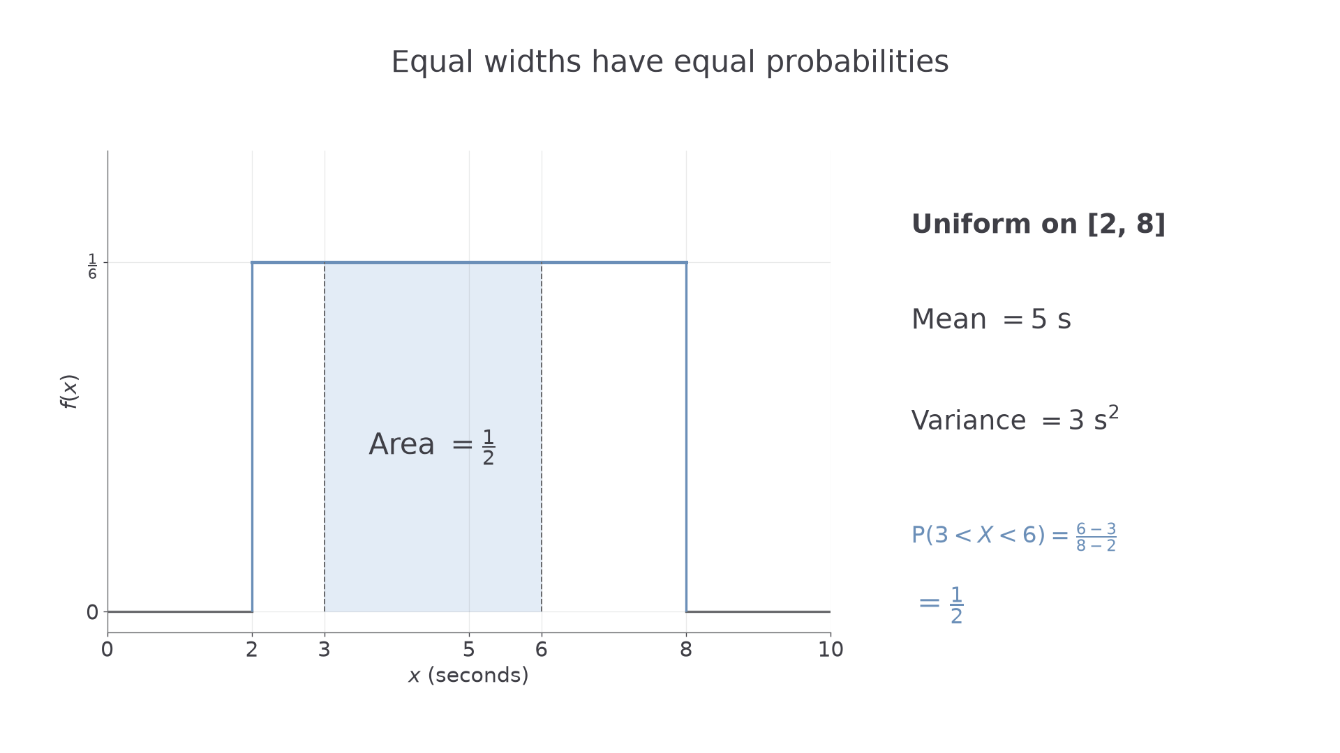
A uniform variable on 2 to 8 has density one sixth, and the interval 3 to 6 has probability one half

Worked example 1: lengths become probabilities

Question. The time $X$ , in seconds, is uniform on $[2,8]$ . Find its mean, variance and $\mathrm{P}(3<X<6)$ .

Plan. Use the midpoint and width for the moments, and divide the event length by the support length.

\begin{aligned} \mathrm{E}(X)&=\frac{2+8}{2}=5 &&\text{midpoint}\\ \mathrm{Var}(X)&=\frac{(8-2)^2}{12}=3 &&\text{squared width over }12\\ \mathrm{P}(3<X<6)&=\frac{6-3}{8-2}=\frac12 &&\text{area of the interval} \end{aligned}

Why this step? The density has the same height everywhere on the support, so an area's probability is proportional to its width.

Answer. Mean $5\,\mathrm{s}$ , variance $3\,\mathrm{s^2}$ , probability $\frac12$ .

Check. The event occupies half the total interval, so its probability is $\frac12$ ; the mean lies at the centre.

Worked example 2 changes one feature: the upper endpoint is unknown, and the mean supplies the missing information. The interval-probability method is unchanged.

Worked example 2: recover a boundary

Question. The time $X$ , in seconds, is uniform on $[2,b]$ , where $b>2$ , and $\mathrm{E}(X)=5$ . Determine $b$ , and hence find $\mathrm{P}(3<X<6)$ .

Plan. Set the midpoint equal to the known mean, then use the recovered support.

\begin{aligned} \frac{2+b}{2}&=5 &&\text{use the mean}\\ b&=8 &&\text{solve}\\ \mathrm{P}(3<X<6)&=\frac{6-3}{8-2}=\frac12 &&\text{use the full width} \end{aligned}

Why this step? The mean locates the midpoint, which determines the other endpoint once one endpoint is known.

Answer. $b=8$ , and the probability is $\frac12$ .

Check. The endpoints $2$ and $8$ are each $3$ seconds from the stated mean $5$ .

A uniform model needs a reason for equal interval probabilities. A bounded measurement is not automatically uniform: if central values occur more often, a rectangular density is unsuitable. A normal model instead describes symmetric concentration around a mean, while the exponential model below is non-negative and skewed.

Watch out

Wrong: $\mathrm{P}(3<X<6)=\frac{6-3}{8}$ for a uniform variable on $[2,8]$ . Right: divide by the support width $8-2$ , not by the upper endpoint. Also $\frac{(b-a)^2}{12}$ is a variance, not a standard deviation.

A fixed upper limit also changes conditional waiting probabilities: surviving close to the endpoint leaves less possible waiting time. The exponential model has a different behaviour.

Exponential probabilities

An exponential waiting time has its greatest density near zero and a decreasing tail that never reaches a fixed deadline.

The parameter $m$ is a positive rate. Larger $m$ concentrates more probability near zero, so it represents a shorter typical wait. If time is measured in minutes, the numerical rate is per minute; converting the time unit also converts the rate.

Exponential distribution

A continuous variable $T$ has an exponential distribution with rate $m>0$ when its density is $f(t)=me^{-mt}$ for $t\ge0$ , and zero for $t<0$ . For example, $m=\frac15$ per minute is a valid positive rate. A negative rate is not valid, and an exponential variable cannot take a negative value.

The density is non-negative, and its improper integral is $\int_0^\infty me^{-mt}\,dt=[-e^{-mt}]_0^\infty=1$ , because $m>0$ . The area to the left of $t\ge0$ is $1-e^{-mt}$ ; the remaining tail is $e^{-mt}$ .

Exponential density

For rate $m>0$ ,

f(t)=me^{-mt}\quad(t\ge0),\qquad f(t)=0\quad(t<0)

In the formula booklet.

Integrating this density supplies the probability rules; the exponential rate and the time must use matching units so that $mt$ has no units.

Exponential c.d.f. and tail

For $T$ exponential with rate $m>0$ ,

F(t)=\begin{cases}0&t<0\\1-e^{-mt}&t\ge0\end{cases}

For $t\ge0$ and $0\le a<b$ ,

\mathrm{P}(T>t)=e^{-mt},\qquad \mathrm{P}(a<T\le b)=e^{-ma}-e^{-mb}

Not in the formula booklet: learn it.

Use the tail when the event says “longer than”; use the c.d.f. when it says “within” or “at most”. The subtraction rule handles an interval.

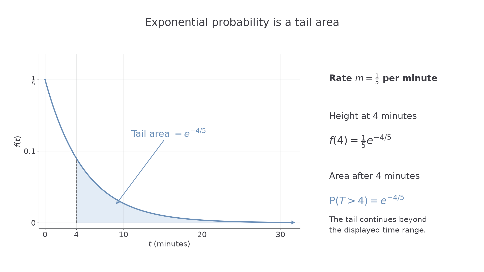
[DIAGRAM: asset_name: An exponential density and a tail probability; asset_slug: h245_5_03_exponential_tail; caption: For rate one fifth per minute, the area after 4 minutes is exp of minus four fifths, not the height of the curve at 4; description: Density graph f(t) equals one fifth times exp of minus t over 5, beginning at height one fifth at t equals 0 and decreasing towards zero. The region to the right of t equals 4 is shaded pale blue and labelled probability T greater than 4 equals exp of minus four fifths. A side panel shows the density height at 4 is one fifth times exp of minus four fifths, distinct from the tail area]
For rate one fifth per minute, the area after 4 minutes is exp of minus four fifths, not the height of the curve at 4

Worked example 3: a tail probability

Question. The time $T$ , in minutes, has an exponential distribution with rate $m=\frac15$ per minute. Find $\mathrm{P}(T>4)$ .

Plan. Use the exponential tail with the time and rate both measured in minutes.

\begin{aligned} \mathrm{P}(T>4)&=e^{-(1/5)4} &&\text{upper tail}\\ &=e^{-4/5} &&\text{simplify the exponent}\\ &=0.449\quad\text{(3 s.f.)} &&\text{evaluate} \end{aligned}

Why this step? The event includes all waits after $4$ , so it is the entire tail area, not the density height at $4$ .

Answer. $e^{-4/5}$ , approximately $0.449$ .

Check. $F(4)=1-e^{-4/5}$ , and the two complementary probabilities add to $1$ .

Worked example 4 changes only the event: the wait must now be between two limits. Remove the tail after the upper limit from the tail after the lower limit.

Worked example 4: an interval probability

Question. For the same rate $m=\frac15$ per minute, find $\mathrm{P}(4<T\le9)$ .

Plan. Subtract the probability of waiting beyond $9$ from the probability of waiting beyond $4$ .

\begin{aligned} \mathrm{P}(4<T\le9)&=\mathrm{P}(T>4)-\mathrm{P}(T>9) &&\text{subtract nested events}\\ &=e^{-4/5}-e^{-9/5} &&\text{use both tails}\\ &=0.284\quad\text{(3 s.f.)} &&\text{evaluate} \end{aligned}

Why this step? Every wait beyond $9$ is also beyond $4$ , so subtracting leaves exactly the required interval.

Answer. $e^{-4/5}-e^{-9/5}$ , approximately $0.284$ .

Check. $F(9)-F(4)=(1-e^{-9/5})-(1-e^{-4/5})$ , the same result; it is smaller than $\mathrm{P}(T>4)$ .

The same rate written per hour would be $12$ per hour. Then $4$ minutes is $\frac1{15}$ hour, and the exponent is still $-12(\frac1{15})=-\frac45$ .

Watch out

Wrong: $\mathrm{P}(T>4)=\frac15e^{-4/5}$ . That is $f(4)$ , a density height. Right: the tail area is $e^{-4/5}$ . Also keep the minus sign: $e^{mt}>1$ for $t>0$ , so it cannot be this probability.

For a general interval, check its position relative to $0$ : the negative part contributes zero probability, just as with any other supported density.

Continue this lesson.

You’re previewing NovaLearn without an account. Create a free account to read the rest.

Create free account

Last Accessed

Pure Core

Statistics

Mechanics

Discrete Mathematics

Additional Pure Mathematics

5.03a - Continuous uniform and exponential distributions

The continuous uniform model

Exponential probabilities

Continue this lesson.

Learn faster with Nova